12.5 Fixed-point iteration and stability
The favorable stability properties of an implicit time-stepping method can be ruined if an unstable numerical method is used to approximately solve the implicit equation that defines it. In particular, such implementations of implicit methods can perform significantly worse for stiff ODEs than the analysis of the previous sections suggest. Indeed, so far all our stability analysis assumed an exact solution of the implicit equation was available at each step of the method.
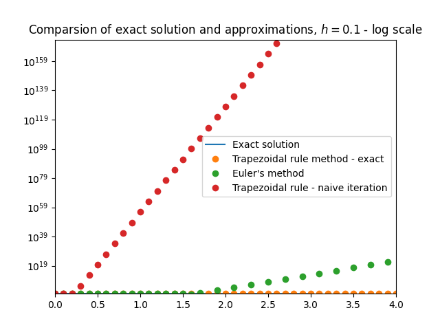
\(\text{ }\)Failure of trapezoidal rule with fixed-point iteration. The only method for solving these implicit equations we have seen so far is the naive fixed-point iteration of Section 9.4. The trapezoidal rule with say ten naive fixed-point iterations amounts to the method \[\begin{array}{ccl} w_{n,0} & = & y_{n},\\ w_{n,m+1} & = & y_{n}+\frac{h}{2}\left(F(t_{n},y)+F(t_{n}+h,w_{n,m})\right),0\le m\le9,\\ y_{n+1} & = & w_{n,10}. \end{array}\tag{12.29}\] Figure Figure 12.9 shows that this method performs even worse than Euler’s method on the stiff ODE ([eq:ch12_stiff_ode_first_example]) from Section 12.1. When we applied the trapezoidal rule method for this ODE in Section 12.1, with the good results shown originally in Figure Figure 12.1 and also included in the present Figure Figure 12.9, the exact solution of the implicit equation was used at each step (the ODE ([eq:ch12_stiff_ode_first_example]) is linear and for linear ODEs the exact solution can be written down explicitly).
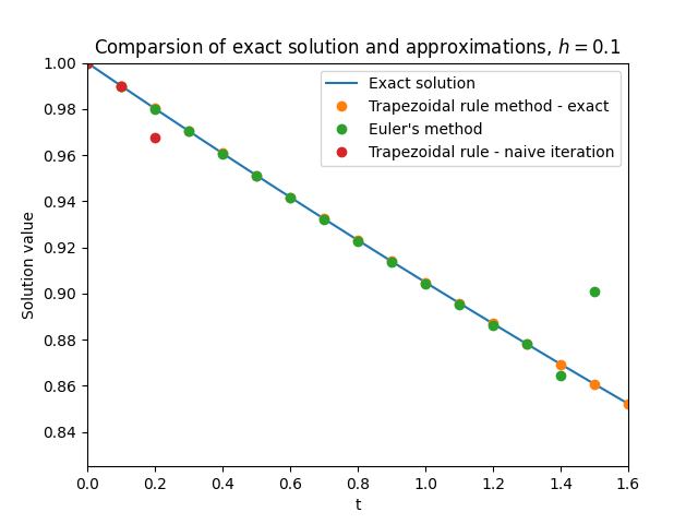
\(\text{ }\)(Small) linear stability region from naive fixed-point iteration. The reason for the failure on display in Figure Figure 12.9 is easy to understand in terms of linear stability region of the method ([eq:ch12_trap_naive_fp]). Unlike the trapezoidal rule with exact solution of the implicit equation, the method ([eq:ch12_trap_naive_fp]) is not \(A\)-stable. To see this we use the framework of Section 12.2, which entails specializing the method ([eq:ch12_trap_naive_fp]) to the scalar linear IVP \(y'(t)=\lambda y,t\ge0,y(0)=1,\) for some \(\lambda\in\mathbb{C},\) to obtain \[\begin{array}{ccl} w_{n,0} & = & y_{n},\\ w_{n,m+1} & = & y_{n}+\frac{h}{2}(\lambda y+\lambda w_{n,m}),0\le m\le9,\\ y_{n+1} & = & w_{n,10}. \end{array}\tag{12.30}\] We can write the fixed-point iteration in the middle line as \[w_{n,m+1}=\beta_{n}+\frac{z}{2}w_{n,m},0\le m\le9,\quad\quad\text{for }\quad\quad z=h\lambda,\] and \(\beta_{n}=y_{n}+\frac{z}{2}y_{n}.\) From this form it easily follows that \[w_{n,m}=\beta_{n}\sum_{i=0}^{m-1}\left(\frac{z}{2}\right)^{i}+\left(\frac{z}{2}\right)^{m}w_{n,0},m\ge0.\tag{12.31}\] It is clear this expression can only be “well-behaved” as \(m\) grows if at least \(\left|\frac{z}{2}\right|<1.\) Arguing more carefully, the form ([eq:ch12_fixed_fp_iter_trap_plus_naive]) implies that \(y_{n+1}=y_{n}r(z)\) and therefore \[y_{n}=y_{0}r(z)^{n},n\ge0,\quad\text{for }\quad r(z)=1+\frac{z}{2}+\sum_{i=2}^{10}\left(\frac{z}{2}\right)^{i}+\left(\frac{z}{2}\right)^{10}.\] The linear stability region is the set \(\mathcal{D}=\left\{ z\in\mathbb{C}:\left|r(z)\right|<1\right\} ,\) the set of \(z\) such that \(y_{n}\to0.\) The precise boundary of \(\mathcal{D}\) is bit complicated, but \(\mathcal{D}\) is clearly contained in a ball of some moderate radius \(R>0\) around the origin. Thus the method is not \(A\)-stable, as opposed to the trapezoidal method with exact implicit solution for which \(\mathcal{D}=\left\{ z\in\mathbb{C}:\mathrm{Re}z<0\right\}\) (recall ([eq:ch12_trap_lsd_difference_eq_sol])-([eq:ch12_trap_lsd_is_neg_imag_half_plane]) and Figure Figure 12.2).
This means that when applied to a system, the method ([eq:ch12_trap_naive_fp_specialized]) is only guaranteed to be stable if \(\left|h\lambda\right|<R\) for all the eigenvalues \(\lambda\) of the Jacobian. More specifically, for the linear stiff ODE ([eq:ch12_stiff_ode_first_example]) with the large “nuisance” eigenvalue \(\lambda=100\) and the smaller eigenvalue \(\lambda=\frac{1}{10}\) (recall ([eq:ch12_stiff_A_eig_decomp])), the stricter condition \(\left|100h\right|<R\) arising from the larger eigenvalue governs stability, rather than the more lenient \(\left|\frac{h}{10}\right|<R\) from the smaller eigenvalue. This is the reason for the divergence of the method when applied with step-size \(h=0.1\) that we see in Figure Figure 12.9.
\(\text{ }\)Newton-Raphson method. To recover \(A\)-stability one needs a more stable numerical method for approximately solving the implicit equation - the natural candidate is the famous Newton-Raphson method. To approximate a root \(\hat{x}\) of a differentiable function \({f:\mathbb{C}^{d}\to\mathbb{C}}\) it takes an initial guess \(x_{0}\in\mathbb{C}\) and then improves it by iterating \[x_{m+1}=x_{m}-\left(J_{f}(x_{m})\right)^{-1}f(x_{m}),\tag{12.32}\] where \(J_{f}(x)=\left(\frac{\partial f_{i}(x)}{\partial x_{j}}\right)_{1\le i,j\le d}\) is the Jacobian matrix of \(f\) at \(x.\) For a scalar function \({f:\mathbb{C}\to\mathbb{C}}\) this simplifies to \[x_{m+1}=x_{m}-\frac{f(x_{m})}{f'(x_{m})}.\]
The Newton-Raphson method is derived from a linear approximation of \(f\) around \(x_{m},\) which in the scalar case reads \[f(x_{m}+\Delta)\approx f(x_{m})+\Delta f'(x_{m}).\tag{12.33}\] Solving the equation \(f(x_{m})+\Delta f'(x_{m})=0\) in \(\Delta\) yields \(\Delta=-\frac{f(x_{m})}{f'(x_{m})}\) suggesting that indeed \(x_{m+1}=x_{m}+\Delta=x_{m}-\frac{f(x_{m})}{f'(x_{m})}\) is a better approximation than \(x_{m}.\) Note that if the function \(f\) is linear then the approximation ([eq:ch12_new_raph_linearization]) is perfect and the solution \(\Delta=-\frac{f(x_{m})}{f'(x_{m})}\) corresponds the true root - in other words the method jumps straight to the exact root \(x_{1}=x_{0}+\Delta\) with \(f(x_{1})=0\) in just one step, regardless of the value of \(x_{0}\) (this holds also in the case \(d\ge2\)). If \(f'(x)\ne0\) (resp. \(J_{f}(x)\) is invertible) and \(f\) is twice-differentiable in a ball \(B\) around a root \(\hat{x},\) then convergence of the method to \(\hat{x}\) is guaranteed if the initial guess \(x_{0}\) lies in \(B\) and satisfies \[M|\hat{x}-x_{0}|<1\quad\quad\text{for}\quad\quad M:=\frac{\sup_{x\in B}|f''(x)|}{\inf_{x\in B}|f'(x)|}.\tag{12.34}\] If so, then furthermore the rate of convergence is faster than with naive fixed-point iteration: it is quadratic in the sense that \(\left|x_{m+1}-\hat{x}\right|\le M\left|x_{m}-\hat{x}\right|^{2},\) which leads to the bound \(|x_{m}-\hat{x}|\le(M|x_{0}-\hat{x}|)^{2^{n}}\) guaranteeing super-exponentially fast convergence. The condition ([eq:c12_newt_raph_conv_cond_scalar]) can be derived by using Taylor’s theorem with remainder to write \[0=f(\hat{x})=f(x_{m})+(\hat{x}-x_{m})f'(x_{m})+(\hat{x}-x_{m})^{2}\frac{f''(\xi)}{2}\] for some \(\xi\in B\) depending on \(x_{n},x,\) reordering as \[f(x_{m})+(\hat{x}-x_{m})f'(x_{m})=-(\hat{x}-x_{m})^{2}\frac{f''(\xi)}{2},\] and then dividing through by \(f'(x_{m})\) to obtain \[\frac{f(x_{m})}{f'(x_{m})}+\hat{x}-x_{m}=-(\hat{x}-x_{m})^{2}\frac{f''(\xi)}{2f'(x_{m})}.\] The l.h.s actually equals \(\hat{x}-x_{m+1},\) and thus we have \[|\hat{x}-x_{m+1}|\le|\hat{x}-x_{m}|^{2}\frac{f''(\xi)}{2f'(x_{m})}\le|\hat{x}-x_{m}|^{2}M,\] (indeed \(x_{m}\in B\) for all \(n\) if \(x_{0}\in B\) and ([eq:c12_newt_raph_conv_cond_scalar]) holds).
\(\text{ }\)Implicit time-stepping methods with Newton-Raphson. The implicit equations for the \(n\)-th step of the implicit numerical time-stepping methods we have seen take the form \[w=\beta_{n}+hg_{n}(w)\] (for the trapezoidal rule method \(\beta_{n}=y_{n}+\frac{h}{2}F(t_{n},y_{n})\) and \(g(w)=\frac{1}{2}F(t_{n+1},w),\) for instance). Applying Newton-Raphson to \(f(w)=w-\beta-hg(w)\) gives \[w_{m+1}=w_{m}-\frac{w_{m}-\beta-hg(w_{m})}{1-hg'(w_{m})},\tag{12.35}\] resp. \(w_{m+1}=w_{m}-(I-hJ_{g}(w_{m}))^{-1}(w_{m}-\beta-g(w_{m})).\) For \(w_{m+1}\) to be well-defined one needs \(|1-hg'(w_{m})|<1\) resp. that \(I-hJ_{g}(w_{n})\) is invertible. Here one aspect of the particular suitability of Newton-Raphson for numerical time-stepping methods can be seen: if the eigenvalues of \(J_{g}(w)\) have negative real part, as one would assume for stability analysis in the spirit of Section 12.2, then the invertibility of \(I-hJ_{g}(w_{n})\) is guaranteed for all \(h\ge0\) - regardless of the magnitudes of the real parts!
The simplest way to start the iteration ([eq:ch12_new_raph_for_time_step_method]) is by setting \[w_{0}=y_{n}.\] A more sophisticated approach is to set \(w_{0}\) to the approximation of \(y(t_{n+1})\) of an explicit method. If one uses an explicit method of the same order as the original implicit method, then the combination of the implicit method and Newton-Raphson retains the order of this original implicit method.
\(\text{ }\)Linear stability domain with Newton-Raphson. If we apply the method ([eq:ch12_new_raph_for_time_step_method]) to a linear equation, then in fact \(w_{1}\) is the exact solution because of the aforementioned behavior of Newton-Raphson for a linear \(f.\) Since the linear stability domain is defined in terms of a linear ODE, it follows that strictly speaking the linear stability region of an implicit method combined with Newton-Raphson is identical to that of the original implicit method with exact solutions. One way wonder if this reflects good stability properties also beyond the strictly linear case, or if it is a special property without wider relevance. A somewhat more satisfying result can be obtained by analyzing the stability of say the trapezoidal rule method combined with Newton-Raphson when applied to the IVP \[y'=\lambda y+ay^{2},\quad t\ge0,\quad y(0)=1,\tag{12.36}\] for some \(a\in\mathbb{C}\) and \(\lambda\in\mathbb{C}\) with \(\mathrm{Re}\lambda<0.\) The explicit solution is \(y(t)=\frac{\lambda e^{t\lambda}}{\lambda+a+ae^{t\lambda}}\) which tends to \(0\) for \(t\to\infty.\) This trapezoidal rule method with \(k\) rounds of Newton-Raphson for this IVP is \[\begin{array}{l} w_{n,0}=y_{n},\\ w_{n,m+1}=w_{n,m}-\frac{w_{n,m}-\beta_{n}-hg(w_{n,m})}{1-hg'(w_{n.m})},0\le m\le k-1,\\ y_{n+1}=w_{n,k}, \end{array}\tag{12.37}\] for \(g(w)=\frac{1}{2}(\lambda w+aw^{2})\) and \(\beta_{n}=y_{n}+\frac{h}{2}(\lambda w+aw^{2}).\) By the convergence condition ([eq:c12_newt_raph_conv_cond_scalar]) for Newton-Raphson, the iteration converges provided \[\left|\frac{2a}{1-h(\lambda+2a)}\right||\hat{w}-w_{0}|<1,\] where \(\hat{w}\) is an exact solution. With the standard assumption \(\mathrm{Re}\lambda<0\) of stability analysis, it typically becomes easier to satisfy this inequality if the magnitude of \(\mathrm{Re}\lambda\) is large! Thus in a stiff system with \(\lambda\) of very different magnitudes, the largest stable step-size should typically not be affected by the presence of an \(\lambda\) with very negative real part.
A matrix is sparse if most of its entries are zero.
\(\text{ }\)Numerical approximation of \(J.\) If one wants to avoid the extra implementation effort of analytically differentiating \(g\) to obtain a formula for the Jacobian, it can be approximated using \[\left(J_{g}(x)\right)_{ij}\approx\frac{g_{i}(x+e_{j}\varepsilon)-g_{i}(x)}{\varepsilon}\] for say \(\varepsilon=\frac{h}{100},\) where \(e_{1},\ldots,e_{d}\) are the standard basis vectors (for very large values of \(d\) this approximation may become problematic, but for moderate values it should be good enough).
\(\text{ }\)Stopping criterion. To maximize stability for stiff problems it is better to iterate “until convergence”, rather than using a fixed number of iterations. One can consider convergence to be achieved to a tolerance tolerance level \(\varepsilon\) for the first iteration such that \(\left|w_{k+1}-w_{k}\right|\le\varepsilon.\)
13 Numerics V: Error control
Picking a step-size is no easy task: one needs to strike the right balance between stability, accuracy and computational efficiency. Error control methods try to handle this task automatically, by adaptively picking \(h\) based on estimates of the error of the current step. The goal is to use a costly small step-size only when absolutely necessary. The user specifies a tolerance parameter \(\delta,\) and the error control method tries to adapt the step-size so that the global error of the approximation is roughly comparable in magnitude to \(\delta.\)
13.1 Embedded Runge-Kutta methods
\(\text{ }\)Local error. Given a one-step method and a particular analytic IVP \(y'=F(t,y)\) and an already computed approximation \(y_{n}\) corresponding to \(t=t_{n},\) we define the local error of the step \(n\to n+1\) as \[y_{n+1}-y(t_{n+1}),\] where \(y\) is the analytic solution to the IVP \(y'=F(t,y),t\in[t_{n},t_{n+1}],y(t_{n})=y_{n}\) (which we assume exists and is unique).
\(\text{ }\)Heuristic estimate of local error. Since the solution \(y\) is analytic it holds for small enough \(h\) that \[y(t_{n+1})=y(t_{n}+h)=\sum_{k=0}^{\infty}\frac{h^{k}}{k!}y^{(k)}(t_{n}).\tag{13.1}\] Restricting attention to Runge-Kutta methods, recall furthermore the expansions of the next approximation \(y_{n+1}\) in \(h,\) around \(y_{n}\) which we derived in Chapter 11 to obtain order conditions. For instance for the general explicit two-stage RK method we obtain in ([eq:ch11_ERK_k=00003D2_set_expansion_final]) the expansion (notation adapted to our current setup) \[y_{n+1}=y(t_{n})+h(b_{1}+b_{2})F+h^{2}b_{2}\left(c_{2}\partial_{t}F+a_{2,1}F\partial_{t}F\right)+O(h^{3}),\tag{13.2}\] where \(F=F(t_{n},y_{n})\) and \(\partial_{t}F=\partial_{t}F(t_{n},y_{n})\) and so on. It is not hard to see that regardless of the number of stages, the tableau and the values of \(t_{n},y_{n},\) there exists a power-series \[y_{n+1}=\sum_{k=0}^{\infty}A_{k}h^{k},\tag{13.3}\] where the \(A_{k}\) depend on the tableau of the method and on \(y(t_{n}),F(t_{n},y_{n}),\partial_{t}F(t_{n},y_{n+1}),\) etc but not on \(h\) (we always have \(A_{0}=y(t_{n}),\) and for explicit two-stage methods \(A_{1},A_{2}\) can be read off from ([eq:ch13_recall_expansion_of_RK_step]) - of instance \(A_{1}=(b_{1}+b_{2})F(t_{n},y(t_{n}))\)). Furthermore the power-series must be convergent for small enough \(h,\) since \(y_{n+1}\) is the composition of analytic functions in \(h\) and therefore analytic. Combing ([eq:ch13_rk_embed_y_expansion]) and ([eq:ch13_rk_embed_y_expansion]) we see that if the RK method is of order \(p,\) then it must hold that \[y_{n+1}=y(t_{n})+\sum_{k=p+1}^{\infty}B_{k}h^{k},\tag{13.4}\] where \(B_{k}=A_{k}-\frac{y^{(k)}(t_{n})}{k!}.\) If \(x_{n+1}\) is computed from \(y_{n}\) using a different Runge-Kutta method which is of order \(p+1,\) then similarly \[x_{n+1}=y(t_{n})+\sum_{k=p+2}^{\infty}C_{k}h^{k},\tag{13.5}\] for small enough \(h,\) for some \(C_{k}\) that do not depend on \(h.\) Subtracting ([eq:ch12_embedd_RK_x_n_meth]) from ([eq:ch12_embedd_RK_y_meth_expansion]) yields \[y_{n+1}-x_{n+1}=B_{p+1}h^{p+1}+O(h^{p+2}).\tag{13.6}\] But at the same time by ([eq:ch12_embedd_RK_x_n_meth]) the error \(y_{n+1}-y(t_{n})\) satisfies \[y_{n+1}-y(t_{n})=B_{p+1}h^{p+1}+O(h^{p+2}),\] with the same leading ordet term on the r.h.s. as ([eq:ch13_embed_RK_meth_diff_expasion]). This justifies the approximation \[\left|y_{n+1}-y(t_{n})\right|\approx\left|y_{n+1}-x_{n+1}\right|\] for the local error at time-step \(n+1.\)
\(\text{ }\)Selecting step-size based on estimated local error. To exploit this estimate to control the step-size of the method generating \(y_{n},\) we compute at each time-step the two estimates \(y_{n+1}\) and \(x_{n+1}\) using their respective Runge-Kutta rules, and define \[\kappa=\left|y_{n+1}-x_{n+1}\right|.\] If \(\kappa\) is below a threshold for the largest acceptable local error, we keep the computed value \(y_{n+1}\) and move on to computing \(y_{n+2}.\) If on the other hand \(\kappa\) is above the threshold, then we reject the approximation \(y_{n+1}\) and instead decrease the step-size. We then compute a new \(y_{n+1}\) (with the smaller step-size), compute \(x_{n+1}\) and the estimate \(\kappa\) and repeat the procedure. Since it is wasteful to use an unnecessarily small step-size, we also increase the step-size if the estimated local error \(\kappa\) falls below an appropriate threshold.
\(\text{ }\)Notation with variable \(h.\) Note that we have quietly abandoned our previous running assumption that \(t_{n}\) denotes \(t_{0}+nh\) for a fixed \(h.\) Instead, we now define \(t_{n}\) recursively, such that if a step with step-size \(h_{n}\) is accepted at step \(n,\) then we set \(t_{n+1}=t_{n}+h_{n}.\) As before \(y_{n}\) denotes the approximation of \(y(t_{n}\)).
\(\text{ }\)Selecting the thresholds. Recall that if a method is of order \(p,\) i.e. has local error which is of order \(O(h^{p+1}),\) then typically the global error is of order \(O(h^{p}).\) We can think of this arising from the accumulation of local errors of order \(O(h^{p+1})\) over \(O(h^{-1})\) time-steps, giving a global error of order \(O(h^{p+1}h^{-1})=O(h^{p}).\) We interpret the tolerance parameter \(\delta>0\) as a desired magnitude of the global error, so the natural thresholds for the local error estimate \(\kappa\) are \[\kappa\le\frac{\delta}{h}\text{ as the condition to accept a step},\] and correspondingly \[\kappa>\frac{\delta}{h}\text{ as the condition to reject a step and decrease }h,\] and say \[\kappa\le\frac{\delta}{10h}\text{ as the condition to increase }h>0,\] (there is no harm in accepting the step before increasing \(h,\) since the estimated error is if anything “too small”).
If the control mechanism is successful in keeping the local error roughly on the order of \(\kappa,\) and if this local error accumulates in a “well-behaved” manner, then we can hope that the global error over a time interval \([t_{0},t_{\max}]\) of fixed length will be roughly of a similar magnitude as \(\delta.\) It goes without saying that there are no guarantees that things work out so nicely, so we should not be surprised if for particular IVPs the behavior of local and global error is very different. But it is reasonable to expect that in many cases, the method is broadly successful in regulating global error.
\(\text{ }\)Computational efficiency. In principle this error control scheme can be applied to any pair of Runge-Kutta method of order \(p\) and order \(p+1\) respectively (or even any other one-step methods of those orders whose step is given by a power-series like ([eq:ch13_embed_erk_step_expansion])). But if we combine some arbitrary pair of RK methods we end up needing essentially double the amount of computational resources as compared to running a method without step-size control. This is typically unacceptable - the error control mechanism should add a comparatively small computational overhead to be useful. The solution is to use two related Runge-Kutta methods, that have almost the same tableau - then we can reuse most of the intermediate computations and the additional overhead of the extra method to compute \(x_{n+1}\) becomes manageable. An example of such a pair of methods are the ones given by the two tableaux \[\begin{array}{c|cc} \boldsymbol{0}\\ \boldsymbol{\frac{2}{3}} & \boldsymbol{\frac{2}{3}}\\ \hline & \frac{1}{4} & \frac{3}{4} \end{array}\quad\quad\text{and}\quad\quad\begin{array}{c|ccc} \boldsymbol{0}\\ \boldsymbol{\frac{2}{3}} & \boldsymbol{\frac{2}{3}}\\ \frac{2}{3} & 0 & \frac{2}{3}\\ \hline & \frac{1}{4} & \frac{3}{8} & \frac{3}{8} \end{array},\tag{13.7}\] with the common elements in bold. The fewer-stage method on the left corresponds to \[\begin{array}{ccl} \xi_{1} & = & y_{n},\\ \xi_{2} & = & y_{n}+\frac{2}{3}hF(t_{n},\xi_{1}),\\ y_{n+1} & = & y_{n}+h\left(\frac{1}{4}F(t_{n},\xi_{1})+\frac{3}{4}F(t_{n}+\frac{2}{3}h,\xi_{2})\right), \end{array}\tag{13.8}\] while the method of the right with one more stage corresponds to \[\begin{array}{ccl} \xi_{1} & = & y_{n},\\ \xi_{2} & = & y_{n}+\frac{2}{3}hF(t_{n},\xi_{1})\\ \xi_{3} & = & y_{n}+\frac{2}{3}hF(t_{n}+\frac{2}{3}h,\xi_{2})\\ x_{n+1} & = & y_{n}+h\left(\frac{1}{4}F(t_{n},\xi_{1})+\frac{3}{8}F(t_{n}+\frac{2}{3}h,\xi_{2})+\frac{3}{8}F(t_{n}+\frac{2}{3}h,\xi_{3})\right). \end{array}\tag{13.9}\] The first two lines of ([eq:ch13_embed_RK_first_example_meth_1]) and ([eq:ch13_embed_RK_first_example_meth_2]) are identical, so the methods use the same values for \(\xi_{1}\) and \(\xi_{2}.\) Thus the combination of both corresponds to \[\begin{array}{ccl} \xi_{1} & = & y_{n},\\ \xi_{2} & = & y_{n}+\frac{2}{3}hF(t_{n},\xi_{1})\\ y_{n+1} & = & y_{n}+h\left(\frac{1}{4}F(t_{n},\xi_{1})+\frac{3}{4}F(t_{n}+\frac{2}{3}h,\xi_{2})\right)\\ \xi_{3} & = & y_{n}+\frac{2}{3}hF(t_{n}+\frac{2}{3}h,\xi_{2})\\ x_{n+1} & = & y_{n}+h\left(\frac{1}{4}F(t_{n},\xi_{1})+\frac{3}{8}F(t_{n}+\frac{2}{3}h,\xi_{2})+\frac{3}{8}F(t_{n}+\frac{2}{3}h,\xi_{3})\right), \end{array}\] whereby the overhead is limited to two last lines. Pairs of Runge-Kutta methods of this type are called embedded Runge-Kutta methods, since we have one RK method embedded inside another. The combined method can be expressed by the combined tableau \[\begin{array}{c|ccc} 0\\ \frac{2}{3} & \frac{2}{3}\\ \frac{2}{3} & 0 & \frac{2}{3}\\ \hline & \frac{1}{4} & \frac{3}{4}\\ \hline & \frac{1}{4} & \frac{3}{8} & \frac{3}{8} \end{array}.\tag{13.10}\] If one deletes the bottom and middle rows, one obtains the smaller left tableau in ([eq:ch13_embed_RK_first_examp_two_tableaus]). If one instead deletes the \(4\)-th row one obtains the larger tableau to the right in ([eq:ch13_embed_RK_first_examp_two_tableaus]).
\(\text{ }\)General embedded RK method. A general embedded RK method is encoded by a tableau of the form \[\begin{array}{c|c} \tilde{c} & \tilde{A}\\ \hline & b^{T}\\ \hline & \tilde{b}^{T} \end{array},\tag{13.11}\] where one of the two bottom rows corresponds to a method of order \(p,\) and the other to method of order \(p+1.\) It is often - but not always - the case that the lower order method has one less stage, and final entry of the weight vector equal to zero. Though in principle possible it is not common practice to embed IRK methods. Any strictly lower triangular \(\tilde{A},\) vector \(\tilde{c}\) with vanishing first entry and arbitrary \(b,\tilde{b}\) gives rise to a correctly formatted embedded RK tableau. The tricky part is finding pairs of methods with the required overlap of the tableau that have the right orders. Deriving the order conditions for standalone RK methods is laborious enough, the order conditions for an embedded method are naturally more involved.
\(\text{ }\)Some common pairs. Luckily there exist reference lists of standard embedded RK methods, such as the Wikipedia page “List of Runge-Kutta methods”. Some common examples are the Heun-Euler method \[\begin{array}{c|cc} 0\\ 1 & 1\\ \hline & \frac{1}{2} & \frac{1}{2}\\ \hline & 1 & 0 \end{array}\] with methods of order \(1\) and \(2,\) the Fehlberg RK1(2) method \[\begin{array}{c|ccc} 0\\ \frac{1}{2} & \frac{1}{2}\\ 1 & \frac{1}{256} & \frac{255}{256}\\ \hline & \frac{1}{512} & \frac{255}{256} & \frac{1}{512}\\ & \frac{1}{256} & \frac{255}{256} & 0 \end{array}\] with methods of order \(2\) and \(3,\) the Bogacki–Shampine method \[\begin{array}{c|cccc} 0\\ \frac{1}{2} & \frac{1}{2}\\ \frac{3}{4} & 0 & \frac{3}{4}\\ 1 & \frac{2}{9} & \frac{1}{3} & \frac{4}{9}\\ \hline & \frac{2}{9} & \frac{1}{3} & \frac{4}{9} & 0\\ & \frac{7}{24} & \frac{1}{4} & \frac{1}{3} & \frac{1}{8} \end{array}\] with orders \(2\) and \(3,\) and the Fehlberg ”RKF45” method \[\begin{array}{c|cccccc} 0\\ \frac{1}{4} & \frac{1}{4}\\ \frac{3}{8} & \frac{3}{32} & \frac{9}{32}\\ \frac{12}{13} & \frac{1932}{2197} & -\frac{7200}{2197} & \frac{7296}{2197}\\ 1 & \frac{439}{216} & -8 & \frac{3680}{513} & -\frac{845}{4104}\\ \frac{1}{2} & -\frac{8}{27} & 2 & -\frac{3544}{2565} & \frac{1859}{4104} & -\frac{11}{40}\\ \hline & \frac{16}{135} & 0 & \frac{6656}{12825} & \frac{28561}{56430} & -\frac{9}{50} & \frac{2}{55}\\ & \frac{25}{216} & 0 & \frac{1408}{2565} & \frac{2197}{4104} & -\frac{1}{5} & 0 \end{array}\] with orders \(4\) and \(5.\)
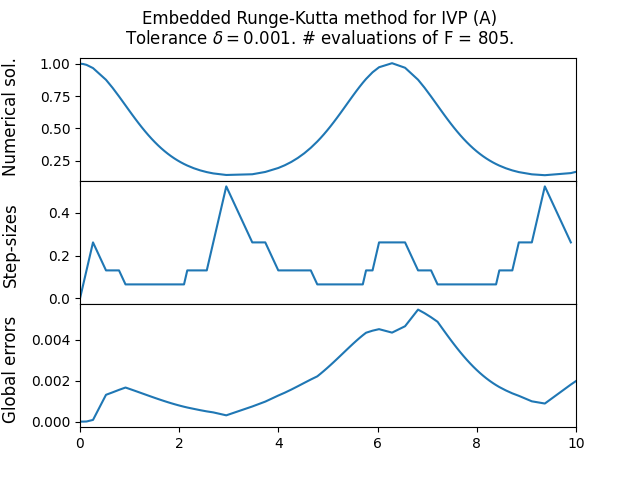
\(\text{ }\)Numerical experiment. Let us now investigate the behavior of the particular embedded RK method ([eq:ch13_emvedd_RK_first_example]) on two benchmark IVPs with explicit solutions. The first one is \[\text{(A)}\quad\quad y'(t)=y\sin(t),\quad t\in[0,10],\quad y(0)=1\] with explicit solution \[y(t)=\exp(\cos(t)-1).\tag{13.13}\] This is a non-stiff ODE.
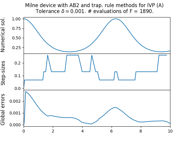
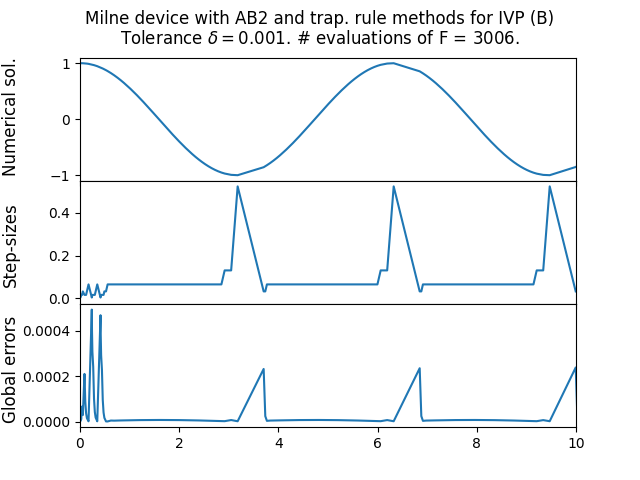
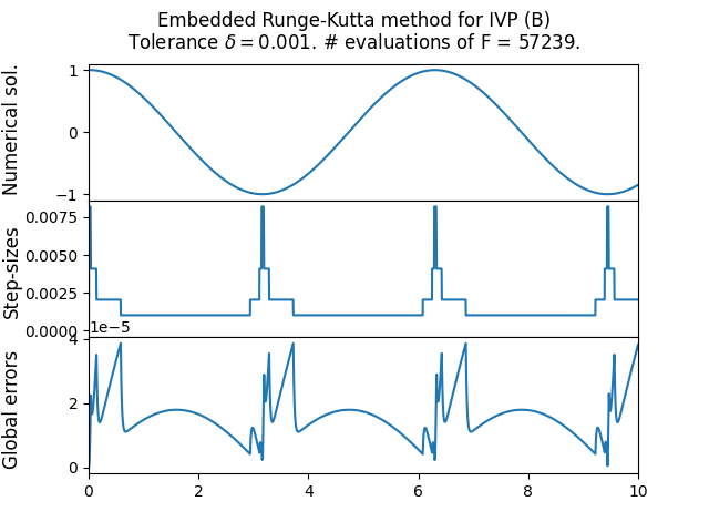
The next is the moderately stiff Curtiss–Hirschfelder equation \[\text{(B)}\quad\quad y'(t)=-50(y-\cos(t)),\quad t\in[0,10],\quad y(0)=1,\] with explicit solution \[y(t)=\frac{2500}{2501}\cos(t)+\frac{50}{2501}\sin(t)+\frac{1}{2501}e^{-50t}.\tag{13.14}\] We use a tolerance parameter of \(\delta=10^{-3}.\) Figure Figure 13.1 shows the results, including the sequence of step-sizes and global error. One can see how the step-size adapts according to the current state of the ODE. Also reported is the number of times the method evaluated the function \(F.\) One sees that for the stiffer ODE the step-sizes become very small, and the number of evaluations of \(F\) is correspondingly large. Indeed embedded RK methods are (essentially always) explicit methods, and as such not the optimal choice for stiff problems. On a positive note, the adaptive step-size means that the method doesn’t catastrophically fail like in Figure Figure 13.1, but instead does a reasonable job in the whole interval, at the cost of a small step-size. For the non-stiff ODE the step-size is kept quite large, and correspondingly the number of evaluations of \(F\) is quite low - nevertheless the magnitude of the global error roughly matches the tolerance parameter \(\delta.\)
13.2 Milne device
The Milne device is an approach to error control for linear multistep methods. It employees two different methods of the same order, and uses the difference in their approximations to estimate the local error. Consider the general form \[\sum_{m=0}^{s}y_{n+m}a_{m}=h\sum_{m=0}^{s}F(t_{n+m},y_{n+m})b_{m}\] for an \(s\)-step multistep method, normalized so that \(a_{s}=1.\)
\(\text{ }\)Meaning of local error. Assume we are applying the method for the step \(n\to n+1.\) If there exists a solution to the ODE defined on \([t_{n},t_{n+s}]\) such that \(y(t_{n+m})=y_{n+m},0\le m\le s-1\) , then one can define the local error as the difference \[y_{n+s}-y(t_{n+s}).\] Of course there is no guarantee that such a solution exists, and then the concept of local error is not well-defined with mathematical precision. This is however not a major problem, we simply assume that such a solution always exists when we heuristically derive the rule of the Milne method, which we can then apply also without such a restrictive assumption.
\(\text{ }\)Expanding the error. Recall that multistep methods can be conveniently characterizes in terms of the polynomials \(\rho(w)=\sum_{m=0}^{s}a_{m}w^{m}\) and \(\sigma(w)=\sum_{m=0}^{s}b_{m}w^{m}.\) The order is determined by the power-series \[\rho(1+\xi)-\sigma(1+\xi)\ln(1+\xi)=\sum_{k=0}^{\infty}c_{k}\xi^{k}.\] Let us assume that the method is of order exactly \(p,\) which by Theorem 10.3 implies that \(c_{0}=\ldots=c_{p}=0,c_{p+1}\ne0.\) Furthermore, for any analytic \(F,\) analytic solution \(y,\) etc. we have the power-series expansion
\[\sum_{m=0}^{s}a_{m}y(t_{n+m})-h\sum_{m=0}^{s}b_{m}F(t_{n+m},y(t_{n+m}))=\sum_{k=p+1}^{\infty}c_{k}h^{k}y^{(k)}(t_{n}),\tag{13.15}\] with the same coefficients \(c_{k}\) (this follows from ([eq:ch_multistep_A_k_B_k_def])-([eq:ch10_A_k_B_k_identity_y])). Let \(y_{n+s}\) be approximation produced by the method when there is a solution \(y(t),t\in[t_{n},t_{n+s}]\) such that \(y(t_{n+m})=y_{n+m},0\le m\le s-1.\) By definition it satisfies \[y_{n+s}-hF(t_{n+s},y_{n+s})+\sum_{m=0}^{s-1}a_{m}y(t_{n+m})-h\sum_{m=0}^{s-1}b_{m}F(t_{n+m},y(t_{n+m}))=0.\] Subtracting this from ([eq:ch13_milne_sol_exp]) we obtain \[y(t_{n+s})-y_{n+s}-h\left(F(t_{n+s},y(t_{n+s}))-F(t_{n+s},y_{n+s})\right)=\sum_{k=p+1}^{\infty}c_{k}h^{k}y^{(k)}(t_{n}).\tag{13.16}\] Since they method is of order \(p\) we already know that \(y(t_{n+s})-y_{n+s}=O(h^{p+1})\) as \(h\downarrow0.\) Since \(F\) is analytic it is Lipschitz in a neighborhood of \((t_{n+s},y(t_{n+s})),\) so for small enough \(h\) we have \(F(t_{n+s},y(t_{n+s}))-F(t_{n+s},y_{n+s})=O\left(\left|y(t_{n+s})-y_{n+s}\right|\right)=O(h^{p+1}).\) Therefore we deduce from ([eq:ch13_milne_after_sub]) that \[y(t_{n+s})-y_{n+s}=c_{p+1}h^{p+1}y^{(p+1)}(t_{n})+O(h^{p+2}).\tag{13.17}\] Now let us fix a different \(\tilde{s}\)-step with coefficients \(\tilde{a}_{m},\tilde{b}_{m},\) which is also exactly of order \(p,\) and use it to compute an approximation \(x_{n+s}\) of \(y(t_{n+s})\) based on the same values of \(y(t_{n+m}),0\le m\le s-1,\) used to produce \(y_{n+s}.\) By the same arguments as above it holds that \[y(t_{n+s})-x_{n+s}=\tilde{c}_{p+1}h^{p+1}y^{(p+1)}(t_{n})+O(h^{p+2})\tag{13.18}\] for a typically different constant \(\tilde{c}_{p+1}.\) Subtracting ([eq:ch13_milne_x_err_xp]) from ([eq:ch13_milne_y_err_xp]) we obtain \[x_{n+s}-y_{n+s}=(c_{p+1}-\tilde{c}_{p+1})h^{p+1}y^{(p+1)}(t_{n})+O(h^{p+2}),\] and assuming that indeed \(c_{p}\ne\tilde{c}_{p},\) we can divide through by \(c_{p+1}-\tilde{c}_{p+1}\) to obtain \[\frac{x_{n+s}-y_{n+s}}{c_{p+1}-\tilde{c}_{p+1}}=h^{p+1}y^{(p+1)}(t_{n})+O(h^{p+2}).\] Plugging this into ([eq:ch13_milne_y_err_xp]) we obtain \[y(t_{n+s})-y_{n+s}=\frac{c_{p+1}}{c_{p+1}-\tilde{c}_{p+1}}(x_{n+s}-y_{n+s})+O(h^{p+2}).\] This justifies the approximation \[\left|y(t_{n+s})-y_{n+s}\right|\approx\frac{\left|c_{p+1}\right|}{\left|c_{p+1}-\tilde{c}_{p+1}\right|}\left|x_{n+s}-y_{n+s}\right|,\] of the local error in terms of the constants \(c_{p+1},\tilde{c}_{p+1}\) and the difference \(\left|x_{n+s}-y_{n+s}\right|.\)
\(\text{ }\)Error control. We can now formulate an adaptive step-size algorithm in analogy with the one for embedded Runge-Kutta methods. Given the current step-size \(h,\) compute \(x_{n+s},y_{n+s}\) using he two different multistep methods, and set \[\kappa=\frac{\left|c_{p+1}\right|}{\left|c_{p+1}-\tilde{c}_{p+1}\right|}\left|x_{n+s}-y_{n+s}\right|.\] Using the tolerance parameter \(\delta>0,\) we accept the step if \(h\kappa\le\delta,\) and otherwise reject it and halve the step-size. If say \(h\kappa\le\frac{\delta}{10}\) , we keep the step but double the step-size before continuing.
\(\text{ }\)Maintaining regular mesh of previous steps. It is however significantly more challenging to implement this approach for multistep methods than for one-step methods. This is because when advancing from a time \(t=t_{n},\) the multistep methods always require \(s\) resp. \(\tilde{s}\) previous approximations, and there must correspond to the regular mesh \(t_{n}-mh,m=0,\ldots,\max(s,\tilde{s}).\) This is not easily compatible with changing step-sizes. The solution is to maintain in addition to the list \(y_{0},y_{1},\ldots\) of accepted approximations for the irregularly spaced times \(t_{0},t_{1},t_{2},\ldots,\) a separate list of previous steps \(\ldots,\ldots,\tilde{y}_{-1},\tilde{y}_{0}\) on the regular mesh corresponding to the current step-size. If a step with same step-size is accepted it is simply added to both list. But if the step-size changes, the list for the regular mesh needs a more comprehensive reorganization.
\(\text{ }\)Doubling step-size. If the the step-size is doubled one can reuse every second value from the list, namely \(\ldots,\tilde{y}_{-4},\tilde{y}_{-2},\tilde{y}_{0}.\) If one ends up with too few previous values to advance the multistep method, an auxiliary method with fewer steps (but preferably with similar stability and order properties) can be used to grow the list until the multistep methods can be applied.
\(\text{ }\)Halving step-size. If the step-size is halved, then one must compute new values corresponding to the midpoints of the previous mesh, for say the most recent \(\max(s,\tilde{s})\) mid-points. This can be done by using polynomial interpolation.
\(\text{ }\)Starting the method. As usual with multistep methods, one needs to apply an auxiliary methods in the beginning until one has the required number of “previous values” - one can for instance implement the whole method using an outer loop that checks if there are enough previous values in the mesh, and if not runs the auxiliary method - this can also provide the corresponding functionality required after doubling the step-size.
\(\text{ }\)Implicit - explicit pair. A very important case of the Milne device uses an implicit method to generate the candidate approximations \(y_{n}.\) Such methods combine the better stability of implicit methods with the adaptability of a variable step-size. There is no reason to use an implicit method to generate the \(x_{n},\) since \(x_{n}\) is discarded as soon as \(\kappa\) has been computed - it is not iterated further. Instead the next \(x_{n}\) is computed from the previous approximations of the implicit method giving \(y_{n}.\)
\(\text{ }\)Fixed-point iteration for implicit method. For approximating the solution of the implicit equation one should use modified Newton-Raphson, so as to not diminish stability too much. Rather than running the implicit method for a large fixed number of time-steps, or until a stringent convergence condition is satisfied, it makes more sense to use the error control mechanism also for the Newton-Raphson iteration. This typically leads to more efficient use of computational resources. A reasonable approach is to run Newton-Raphson iteration for say \(10\) rounds. If a convergence condition of the form \(|w_{10}-w_{9}|\le\varepsilon\) has been achieved (for a \(\varepsilon\) significantly smaller than \(\delta/h\)), set the next \(y_{n+s}\) to \(w_{10}.\) If the convergence condition is not satisfied, reject the step, halve the step-size and try again, as when the condition \(h\kappa\ge\delta\) is triggered.
\(\text{ }\)The TR-AB2 pair. Let us now consider a concrete example of the Milne device, using the one-step implicit second order trapezoidal rule method as the main method, and the explicit two-step second order Adams-Bashforth method for computing the error estimate. The explicit Adams-Bashforth method is \[x_{n+1}=x_{n}+h\left(\frac{3}{2}F(t_{n},x_{n})-\frac{1}{2}F(t_{n-1},x_{n-1})\right)\tag{13.19}\] and the implicit trapezoidal rule method is \[y_{n+1}-y_{n}=h\left(\frac{1}{2}F(t_{n},x_{n})+\frac{1}{2}F(t_{n-1},x_{n-1})\right).\tag{13.20}\] The method ([eq:ch13_milne_AD]) corresponds to \(\rho(w)=w^{2}-w\) and \(\sigma(w)=\frac{3}{2}w-1,\) yielding the power-series \[\rho(1+\xi)-\sigma(1+\xi)\log(1+\xi)=\frac{5}{12}\xi^{3}+O(\xi^{4}),\] while the method ([eq:ch13_milne_trap]) corresponds to \(\rho(w)=w-1\) and \(\sigma(w)=\frac{w+1}{2}\) with power-series \[\rho(1+\xi)-\sigma(1+\xi)\log(1+\xi)=-\frac{1}{12}\xi^{3}+O(\xi^{4}).\] Thus the constants \(c_{p+1},\tilde{c}_{p+1}\) are given by \(c_{p+1}=\frac{5}{12}\) and \(\tilde{c}_{p}=-\frac{1}{12}.\)
We choose to at least three properly spaced “previous values” \(\tilde{y_{2}},\tilde{y_{1}},\tilde{y_{0}}\) corresponding to the mesh \(\left\{ t-2h,t-h,t\right\} .\) This means that after halving \(h\) the old list \(\tilde{y_{2}},\tilde{y_{1}},\tilde{y_{0}}\) now corresponds to the mesh \(\left\{ t-4h,t-2h,t\right\}\) (for the new halved values of \(h\)). The new list is \(\tilde{y_{1}},\tilde{y}_{{\rm mid}},\tilde{y_{0}},\) where \(\tilde{y}_{{\rm mid}}\) approximates \(y(t-h).\) A polynomial interpolation based on all the values \(\tilde{y_{2}},\tilde{y_{1}},\tilde{y_{0}}\) of the old list prescribes that \[\tilde{y}_{{\rm mid}}=\frac{3}{8}\tilde{y}_{0}+\frac{6}{8}\tilde{y}_{1}-\frac{1}{8}\tilde{y}_{2}.\] We have now provided all the information needed to implement the algorithm.
\(\text{ }\)Results when applied to benchmark ODEs. Figure Figure 13.1 shows the results when this algorithm is applied to the non-stiff ODE (A) and the moderately stiff (B). For the non-stiff problem it achieves global error close to the target magnitude, as does the embedded RK method, while using more function evaluations that the latter method. For the stiffer ODE this implicit method can make do with much larger step-sizes than the explicit embedded RK method, and correspondingly uses many fewer function evaluations.