3.9 Implicit solutions
As mentioned in Chapter 1 Section 1.4, there are many differential equations whose solutions can not be written as explicit closed form formulas. Some of these however admit a closed form implicit solution formula.
Finding implicit solution formulas.
Let us solve the ODE \[(y^{4}-1)y'=1.\tag{3.96}\] It is separable, and integrating both sides gives \[\frac{y^{5}}{5}-y=t+c.\tag{3.97}\] If we could solve for \(y\) we could obtain an explicit solution formula. But this the l.h.s. is a quintic polynomial equation in \(y,\) and there is no closed form formula for its roots valid for arbitrary values of the r.h.s. However ([eq:ch3_implicit_sol_first_ex_sol]) is an implicit formula for the solutions: any solution must satisfy this relation for some constant \(c\) (the original ODE ([eq:ch3_implicit_sol_first_ex_ODE]) is of course also relation that all solutions must satisfy, but it involves the derivative - the relation ([eq:ch3_implicit_sol_first_ex_sol]) does not). Equation ([eq:ch3_implicit_sol_first_ex_sol]) give the solutions in the form of a one parameter implicitly defined family of curves, parameterized by the constant \(c.\)
We call ([eq:ch3_implicit_sol_first_ex_sol]) an implicit solution of the ODE ([eq:ch3_implicit_sol_first_ex_ODE]). In general if one can find a function \(G(t,y)\) (possibly parameterized by one or more parameters) such that the solutions of the ODE are those functions \(y(t)\) that satisfy \[G(t,y(t))=0,\quad\quad t\in I,\tag{3.98}\] then we call ([eq:ch3_implicit_sol_general_sol]) an implicit solution of the ODE. Note the similarity to but crucial difference from the general form ([eq:ch3_implicit_eq]) of an implicit ODE (namely absence of derivatives in ([eq:ch3_implicit_sol_general_sol])). When solving first order ODEs using separability one always obtains implicit solutions - indeed the general formula ([eq:ch3_thm_sep_sol]) is in implicit form. Depending on the form of these implicit solutions they can then sometimes be turned into explicit solutions, but often the implicit solution formula is the best one can do.
Sometimes even when an explicit solution is available, the implicit solution formula is nicer. Compare for instance \[x^{2}+y^{2}=1\text{ (implicit)}\quad\quad\text{ to }y=\pm\sqrt{1-x^{2}}\text{ (explicit)}.\tag{3.100}\] The former is a nicer formula and also more readily identifiable as the equation for a circle. Furthermore implicit solutions like \[y^{3}-y=t+c\quad\quad\text{ or }\quad\quad y^{4}-y=t^{5}+c\tag{3.101}\] can in principle be turned into explicit solutions since cubic and quartic equations can be solved explicitly, but the formulas for the solution are so impractical that they are rarely useful - leaving the solution in the form ([eq:ch3_implicit_nicer_than_explicit_2]) is usually preferable.
If one can obtain an implicit solution of an ODE it is often easy to solve a corresponding IVP.
Let us solve the ODE \[(y^{4}-1)y'=1.\tag{3.96}\] It is separable, and integrating both sides gives \[\frac{y^{5}}{5}-y=t+c.\tag{3.97}\] If we could solve for \(y\) we could obtain an explicit solution formula. But this the l.h.s. is a quintic polynomial equation in \(y,\) and there is no closed form formula for its roots valid for arbitrary values of the r.h.s. However ([eq:ch3_implicit_sol_first_ex_sol]) is an implicit formula for the solutions: any solution must satisfy this relation for some constant \(c\) (the original ODE ([eq:ch3_implicit_sol_first_ex_ODE]) is of course also relation that all solutions must satisfy, but it involves the derivative - the relation ([eq:ch3_implicit_sol_first_ex_sol]) does not). Equation ([eq:ch3_implicit_sol_first_ex_sol]) give the solutions in the form of a one parameter implicitly defined family of curves, parameterized by the constant \(c.\)
\(\text{ }\) Information about solution from implicit form Implicit solution formulas can give a lot of information about the solutions.
Let us solve the ODE \[(y^{4}-1)y'=1.\tag{3.96}\] It is separable, and integrating both sides gives \[\frac{y^{5}}{5}-y=t+c.\tag{3.97}\] If we could solve for \(y\) we could obtain an explicit solution formula. But this the l.h.s. is a quintic polynomial equation in \(y,\) and there is no closed form formula for its roots valid for arbitrary values of the r.h.s. However ([eq:ch3_implicit_sol_first_ex_sol]) is an implicit formula for the solutions: any solution must satisfy this relation for some constant \(c\) (the original ODE ([eq:ch3_implicit_sol_first_ex_ODE]) is of course also relation that all solutions must satisfy, but it involves the derivative - the relation ([eq:ch3_implicit_sol_first_ex_sol]) does not). Equation ([eq:ch3_implicit_sol_first_ex_sol]) give the solutions in the form of a one parameter implicitly defined family of curves, parameterized by the constant \(c.\)
(Continuation of Example 3.35) Let us solve the IVP \[(y^{4}-1)y'=1,\quad\quad t\ge0,\quad\quad y\left(\frac{2}{5}\right)=2.\tag{3.102}\] Previously in ([eq:ch3_implicit_sol_first_ex_sol]) we obtained the parametric family of solutions \[\frac{y^{5}}{5}-y=t+c.\tag{3.103}\] The IVP ([eq:ch3_implicit_sol_first_ex_ODE_IVP]) requires that \(y=2\) when \(t=\frac{2}{5}\) , and plugging this into ([eq:ch3_implicit_sol_first_ex_sols_repeat]) we see that the solution must be the member of the family whose \(c\) satisfies \[\frac{2^{5}}{5}-2=\frac{2}{5}+c.\] In other words it must hold that \(c=\frac{2^{5}}{5}-2-\frac{2}{5}=4.\) Thus \[\frac{y^{5}}{5}-y=t+4.\tag{3.104}\] is an implicit solution to the IVP.
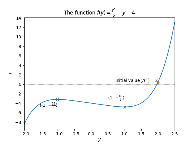
The solution curve has this general shape because for \(y\) large the term \(\frac{y^{5}}{5}\) “dominates” (it’s much larger than \(y\)), causing the steep divergence to \(\infty\) for \(y\to\infty\) and \(-\infty\) for \(y\to-\infty,\) while for small \(y\) the term \(-y\) “dominates” (it’s much larger than \(y^{5}\)) - the term \(-4\) is of course just a constant shift.
That there are exactly two critical points can be verified rigorously by noting that the slope of the curve is given by \[f'(y)=y^{4}-1,\] which is a polynomial with exactly two real roots \(y=\pm1.\) Furthermore for \(y=\pm1\) the value of \(t\) is \(\frac{y^{5}}{5}-y-4=\pm(\frac{1}{5}-1)-4=-4\mp\frac{4}{5},\) so the locations of the critical points at \((y,t)=(-1,-\frac{24}{5})\) and \((y,t)=(1,-\frac{16}{5})\) are explicit.
If we now flip the axes, we obtain a plot of the solution \(y(t)\) as a function of \(t\)! This amounts to mirroring the plot in Figure 3.13 along the diagonal:
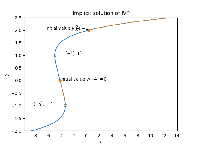
From this we see for instance that the solution of the IVP exists for all \(t\ge t_{0}=\frac{2}{5},\) and is increasing.
With the modified IVP condition \(y(-4)=0\) the implicit solution curve is the same (since the point \(y=0,t=-4\) lies on this curve, for the same \(c=4\)), but we see from the plot that the solution \(y(t),t\ge t_{0}=-4\) is decreasing and only exists up (and not including) \(t=-\frac{24}{5}\) which corresponds to the left critical point of Figure (Figure 3.13). With the flipped axes the critical points turns into a degenerate slope of “\(-\infty\)”, so as the solution to this IVP approaches \(t=-4\) the derivative \(y'(t)\) diverges to \(-\infty\) , so that the solution is no longer well-defined for \(t\ge-\frac{24}{5}.\)
Computer algebra systems can plot implicitly defined curves. Try entering
“contour plot y**5/5 - y = t + 4” into wolframalpha.com.
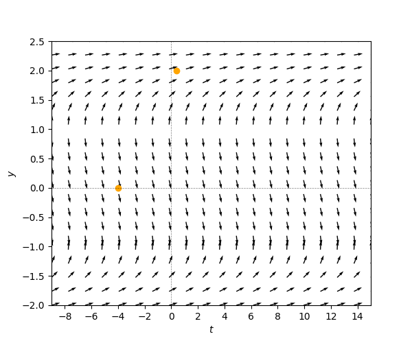
With additional effort of the imagination the qualitative picture of the previous example could also have been read off from the tangent field (below). The coordinate \(y=-1\) where the solution to the second IVP ends could also be deduced from only the formula \((y^{4}-1)y'=1\) for the ODE, but the value \(t=-\frac{24}{5}\) and of course the solution curve can only be read off approximately.
Find an implicit solution to the IVP \[(e^{y}-2)y'=2t,\quad\quad y(-1)=0.\] Sketch the solution. What is the longest interval \(I\) of the form \(I=[-1,t_{\max})\) on which your solution exists?
(Solution on next page).
Solution:The ODE is separable and can be written as \[e^{y}y'-2y'=2t.\] Integrating both sides we obtain the implicit family of solutions \[e^{y}-2y=t^{2}+c.\] Plugging in \(y=0\) and \(t=-1\) we obtain the equation \[e^{0}-2\cdot0^{2}=(-1)^{2}+c,\] for the \(c\) that corresponds to the solution of the IVP. This gives \(c=0,\) so the IVP is solved by the implicit solution \[e^{y}-2y=t^{2}.\] This cannot be solved explicitly for \(y,\) but solving for \(t\) yields \[t=\pm\sqrt{e^{y}-2y}.\] Plotting \(f_{+}(y)=\sqrt{e^{y}-2y}\) and \(f_{-}(y)=-\sqrt{e^{y}-2y}\) we obtain:
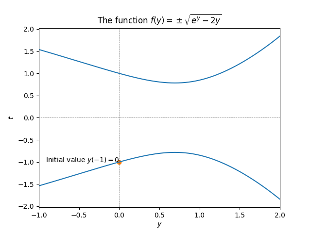
The initial point lies on the curve \(-\sqrt{e^{y}-2y}.\)
Switching the axes and mirroring the plot we obtain a plot of the solution curve \(y(t)\) as a function of \(t\):
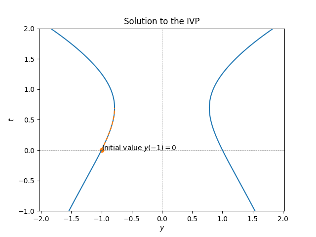
We see that the solution of IVP increases after \(t_{0}=-1\) and stops being a valid solution at a point which corresponds to the critical point in Figure Figure 3.16. This is the point that satisfies \[f_{-}'(y)=-\frac{1}{2}\frac{e^{y}-2}{\sqrt{e^{y}-2y}}=0,\] and thus has \(y=\ln2,\) which gives \[t_{\max}:=-\sqrt{e^{\ln2}-2\ln2}=-\sqrt{2-2\ln2}=-2\sqrt{1-\ln2}=-1.0788.......\] The maximal interval \(I\) is \(I=[-1,t_{\max})\) for this \(t_{\max}.\)
Practice finding implicit solutions using the following quiz.
3.10 Exact equations
Exact equations are a class of first order ODEs whose solutions can be written more-or-less explicitly.
Consider \[y'=-\frac{2xy}{x^{2}+2y}.\tag{3.109}\] This ODE is
not linear: it is equivalent to \(x^{2}y'+2yy'=-2xy\) and the term \(yy'\) makes in non-linear,
not separable: one can’t separate \(x\) and \(y\) in the term \(x^{2}+2y.\)
But the ODE has another interesting property that can be seen from the form \[(x^{2}+2y)y'+2xy=0.\] Namely \[x^{2}+2y=\partial_{y}\left(x^{2}y+y^{2}\right),\] and \[2xy=\partial_{x}\left(x^{2}y+y^{2}\right).\] Thus the ODE is equivalent to \[\partial_{y}F(x,y)y'+\partial_{x}F(x,y)=0\quad\quad\text{ for }\quad\quad F(x,y)=x^{2}y+y^{2}.\tag{3.110}\] Recall the law of total derivative: for a differentiable function \(G(u,v)\) and differentiable functions \(a(x),b(x)\) the derivative of the function \(x\to G(a(x),b(x))\) is given by \[\frac{d}{dx}G(a(x),b(x))=a'(x)\partial_{u}G(a(x),b(x))+b'(x)\partial_{v}G(a(x),b(x)).\] Using this we see that the l.h.s of ([eq:ch3_exact_equations_first_example]) is \(\frac{d}{dx}F(x,y(x))\)! Thus the ODE ([eq:ch3_exact_equations_first_example_ODE]) is equivalent to \[\frac{d}{dx}F(x,y(x))=0,\] and we integrate both sides we arrive at the implicit solution \[F(x,y(x))=c,\] for the ODE, or in this particular case \[x^{2}y+y^{2}=c.\]
First order ODEs for which such a function \(F(y,x)\) exists are called exact equations.
Let \(I,I_{y}\) be intervals and let \(A,B:I\times I_{y}\to\mathbb{R}\) be functions. The ODE \[y'(x)A(x,y)+B(x,y)=0,\] is called an exact ODE if there is a differentiable \(F(x,y)\) such that \(A(x,y)=\partial_{y}F(x,y)\) and \(B(x,y)=\partial_{x}F(x,y).\)
Consider the ODE \[(x+1)y'+y=0.\tag{3.111}\] To see if this is exact we have to investigate if we can find a function \(F(x,y)\) with \(\partial_{x}F(x,y)=y\) and \(\partial_{y}F(x,y)=x+1.\) If \(\partial_{x}F(x,y)=y\) the integrating both sides in \(x,\) leaving \(y\) fixed (i.e. without considering the relationship between \(y\) and \(x,\) viewing \(y\) simply as a constant) we see that this \(F\) would have to have the form \[F(x,y)=xy+c,\tag{3.112}\] where here \(c\) is allowed to be an expression that depends on \(y.\) Similarly if \(F\) satisfies \(\partial_{y}F(x,y)=x+1\) then it must have the form \[F(x,y)=yx+y+c',\tag{3.113}\] where \(c'\) can depend on \(x.\) Is there some \(F\) that matches both ([eq:ch3_exact_second_example_ODE_pattern_1]) and ([eq:ch3_exact_second_example_ODE_pattern_2]). Yes, it is not hard to see that \(F(x,y)=xy+y=(x+1)y\) does! Indeed for this \(F\) it holds that \(\partial_{x}F(x,y)=y\) and \(\partial_{y}F(x,y)=x+1,\) so the ODE ([eq:ch3_exact_second_example_ODE]) is equivalent to \[y'\partial_{y}F(x,y)+\partial_{x}F(x,y)=0,\] and therefore also to \[\frac{d}{dx}F(x,y(x))=0.\] Thus \[F(x,y(x))=c,\] or equivalently \[(x+1)y(x)=c\] or \[y(x)=\frac{c}{x+1},\tag{3.114}\] are solutions.
Note that the ODE ([eq:ch3_exact_second_example_ODE]) is equivalent to the first order linear ODE \[y'=-\frac{y}{1+x},\] (as long as \(x\ne1\)). Check that you recover the family of solutions ([eq:ch3_exact_second_example_ODE_sol]) by using the methods of Section 3.5.
If an ODE of the form
\[y'A(x,y)+B(x,y)=0\] is exact, then since \(\partial_{xy}F(x,y)=\partial_{yx}F(x,y)\) for any differentiable \(F,\) it must hold that \[\partial_{x}A(x,y)=\partial_{xy}F(x,y)=\partial_{yx}F(x,y)=\partial_{y}B(x,y).\] Thus if \(\partial_{y}B(x,y)\ne\partial_{x}A(x,y)\) then the ODE is not exact. There is a converse of this statement but we omit it. In practice, if \(\partial_{y}B(x,y)=\partial_{x}A(x,y)\) it is usually easy to find \(F\) such that \(\partial_{y}F(x,y)=A(x,y)\) and \(\partial_{x}F(x,y)=B(x,y),\) thus proving that the ODE is exact.
Which of the following ODEs are exact?
(a) \(y'=-\frac{2x+y}{x+2y}\)
(b) \(y'(3x+y)+5xy+4y=0.\)
(c) \(2x^{2}yy'+2xy^{2}+2=0\)
(c) \(y'(x\cos(y)+1)+\cos ydx.\)
(a) We rewrite (a) as \[y'(x+2y)+2x+y=0.\] We compute \(\partial_{y}\left\{ x+2y\right\} =2\) and \(\partial_{x}\{2x+y\}=2.\) Since these coincide the ODE could be exact. Indeed also \(\int(2x+y)dx=x^{2}+xy+c\) (for \(y\) fixed) and \(\int(x+2y)dy=xy+y^{2}+c,\) which suggests that \(F(x,y)=x^{2}+y^{2}+xy\) is the function we need to show that (a) is exact. Indeed \(\partial_{y}F(x,y)=x+2y\) and \(\partial_{x}F(x,y)=2x+y,\) so (a) is exact.
(b) We compute \(\partial_{x}(3x+y)=3\) and \(\partial_{y}(5xy+4y)=5x.\) These don’t coincide, so (b) is not exact.
(c) We compute \(\partial_{x}(2x^{2}y)=4xy\) and \(\partial_{y}(2xy^{2}+2)=4xy\) which coincide, so the equation could be exact. And indeed \(\int2x^{2}ydy=x^{2}y^{2},\) and setting \(F(x,y)=x^{2}y^{2}+2x\) we obtain \(\partial_{y}F(x,y)=2x^{2}y\) and \(\partial_{x}F(x,y)=2xy^{2}+2,\) so (c) is exact.
(d) We compute \(\partial_{x}(x\cos(y)+1)=\cos(y)\) and \(\partial_{y}\cos y=-\sin(y)\) which don’t agree, so (d) cannot be exact.
3.11 Integrating factors
Some ODE that are not exact, but can be made exact by multiplying with an appropriate factor. Such factors are called integrating factors.
Consider the ODE \[y'+y=0.\tag{3.115}\] It has the form \(y'A(x,y)+B(x,y)\) for \(A(x,y)=1\) and \(B(x,y)=y.\) This is not exact, since \(\partial_{x}\{1\}=0\) and \(\partial_{y}\{y\}=1.\) But if we multiply by \(e^{x}\) then the ODE becomes \[e^{x}y'+e^{x}y=0,\] and \[\partial_{x}\left\{ e^{x}y\right\} =e^{x}y\text{ and }\partial_{y}\left\{ e^{x}y\right\} =e^{x},\] so this ODE is exact and solved by \[e^{x}y(x)=c,\] or in other words \[y(x)=ce^{-x}.\]
The ODE ([eq:ch3_int_fact_example_1]) is a first order linear autonomous ODE. Check that the methods of Section 3.2 yield the same solutions.
There is no universal method for finding integrating factors, except for certain specific classes of ODEs. One way to proceed is to try go guess expressions that when differentiated in \(x\) or \(y\) produce something equal to or at least resembling terms of ODE. One tries to compensate any extraneous terms that appear when doing so in such way that one ends up with the ODE one is trying multiplied by an expression. If found, this expression is the integrating factor.
Consider the ODE \[y'(3xy^{2}+4x^{2}y)+(2y^{3}+6xy^{2})=0\tag{3.116}\] Lets look for an integrating factor. We do so by looking for an \(F\) such that \(y'\partial_{x}F(x,y)+\partial_{y}F(x,y)=0\) is a multiple of the ODE.
For clarity lets give the terms
labels. \[y'(\underset{I}{\underbrace{3xy^{2}}}+\underset{II}{\underbrace{4x^{2}y}})+(\underset{III}{\underbrace{2y^{3}}}+\underset{IV}{\underbrace{6xy^{2}}})=0.\tag{3.117}\] Let start with the term \(I.\) This should arise when applying \(\partial_{y}\) to an expression \(F(x,y).\) It could arise from \(xy^{3}\) since \(\partial_{y}\{xy^{3}\}=3xy^{2}.\) Lets try this scenario out by making the ansatz \(F(x,y)=xy^{3}.\) This \(F(x,y)\) has total derivative \[\frac{d}{dx}\left\{ xy^{3}\right\} =y'\underset{=I\checkmark}{\underbrace{(3xy^{2})}}+\underset{\text{ close to }III....}{\underbrace{y^{3}}}.\] We recover \(I,\) and from applying \(\partial_{x}\) almost \(III\) too! However, a factor \(2\) is missing. If we had started with \(x^{2}y^{3}\) we would get this factor \(2\) after applying \(\partial_{x},\) resulting in \(2xy^{3}.\) But this term has a factor \(x\) not present in \(III\) in ([eq:ch3_int_factors_first_example_finding_labelled]). We can make things consistent by introducing an extra \(x\) that we multiply by all terms in ([eq:ch3_int_factors_first_example_finding_labelled]) , arriving at \[y'(\underset{I'}{\underbrace{3x^{2}y^{2}}}+\underset{II'}{\underbrace{4x^{3}y}})+(\underset{III'}{\underbrace{2xy^{3}}}+\underset{IV'}{\underbrace{6x^{2}y^{2}}})=0.\] Note that this ODE has the same solutions as ([eq:ch3_int_factors_first_example_finding]). We should now recheck our ansatz, or rather our new modified ansatz \(F(x,y)=x^{2}y^{3}.\) Now the total derivative is \[\frac{d}{dx}\{x^{2}y^{3}\}=y'\underset{=I'\checkmark}{\underbrace{(3x^{2}y^{2})}}+\underset{=III'\checkmark\checkmark}{\underbrace{2x^{2}y^{3}}.}\] Note that the first term still coincides with \(I',\) and now also the second term from the total derivative of \(x^{2}y^{3}\) reproduces the term \(III'\) of the modified ODE perfectly! That’s good news. Can we also reproduce the remaining \(II',IV'\)? We note that \(II'\) has one more power of \(x\) and \(IV'\) one more power of \(y,\) just as for \(I',III'.\) For \(I',III'\) this happened from applying \(\partial_{y}\) resp. \(\partial_{x}\) to a term of the form \(x^{a}y^{b}.\) The most straight-forward scenario would be simply \(x^{3}y^{2}\): lo and behold \[\frac{d}{dx}\{x^{3}y^{2}\}=y'\underset{=\frac{1}{2}\times II'}{\underbrace{(2x^{3}y)}}+\underset{=\frac{1}{2}\times IV'}{\underbrace{3x^{2}y^{2},}}\] which are the terms \(I'',IV'\) up to a factor \(2.\) Thus we have finally arrived at \[\begin{array}{ccc} \frac{d}{dx}\left\{ x^{2}y^{3}+2x^{3}y^{2}\right\} & = & y'\left(\underset{=I'\checkmark}{\underbrace{3x^{2}y^{2}}}+\underset{=I''\checkmark}{\underbrace{2x^{2}y}}\right)+\underset{=III'\checkmark}{\underbrace{2xy^{3}}}+\underset{=IV'\checkmark}{\underbrace{6x^{2}y^{2}}}\\ & = & x\left\{ y'\left(\underset{=I\checkmark}{\underbrace{3xy^{2}}}+\underset{=I'\checkmark}{\underbrace{2xy}}\right)+\underset{=III\checkmark}{\underbrace{2y^{3}}}+\underset{=IV\checkmark}{\underbrace{6xy^{2}}}\right\} . \end{array}\] Note that the r.h.s. is the ODE ([eq:ch3_int_factors_first_example_finding]) multiplied by \(x,\) and is shown here to be an exact equation with \(F(x,y)=xy^{3}+2x^{3}y^{2}.\) Thus \(x\) is an integrating factor of ([eq:ch3_int_factors_first_example_finding_labelled]) and it is solved by \[x^{2}y^{3}+2x^{3}y^{2}=c.\]
Consider the ODE \[y'\frac{x^{2}}{y}+(x\ln\left|xy\right|+x)=0.\] Let us try to find an integrating factor.
Interestingly from the point of view of exactness, the term that should come from \(\partial_{y}\) has a factor \(\frac{1}{y}\) while the one that should come from \(\partial_{x}\) has \(\ln|y|\) (recall that \(\partial_{y}\ln|y|=\frac{1}{y}\)). Let’s separate \(\ln|xy|=\ln|x|+\ln|y|\) and write \[\underset{I}{\underbrace{y'\frac{x^{2}}{y}}}+\underset{II}{\underbrace{x\ln|y|}}+\underset{III}{\underbrace{x\ln\left|x\right|}}+\underset{IIIV}{\underbrace{x}}=0,\tag{3.118}\] and start by trying to reproduce the term \(I\) in our total derivative, which leads us to take the total derivative of \(x^{2}\ln|y|\): \[\frac{d}{dx}\left\{ x^{2}\ln|y|\right\} =y'\underset{=I\checkmark}{\underbrace{\frac{x^{2}}{y}}}+\underset{\text{almost }II...}{\underbrace{2x\ln|y|}}.\] We did get the term \(I,\) and almost the term \(III,\) just with the wrong prefactor \(+2.\) To get rid of the factor we should start with \(x\ln|y|,\) whose total derivative is \[\frac{d}{dx}\left\{ x\ln|y|\right\} =y'\left\{ \frac{x}{y}\right\} +\ln|y|.\tag{3.119}\] But then we have lost a factor \(x\) in each term \(I,II.\) However, dividing all terms in ([eq:ch3_int_factor_second_example_ODE_labelled]) we obtain \[\underset{I'}{\underbrace{y'\frac{x}{y}}}+\underset{II'}{\underbrace{\ln|y|}}+\underset{III'}{\underbrace{\ln\left|x\right|}}+\underset{IIIV'}{\underbrace{1}}=0.\tag{3.120}\] Now the total derivative ([eq:ch3_int_factor_second_example_tot_derivative_lower_power_x]) does reproduce \(I',II'\) perfectly. It remains to account for \(III',IIIV'.\) But these don’t depend on \(y,\) so if have and \(f(x)\) such that \(f'(x)=\ln|x|+1\) we just add this to our \(F(x,y)\) and we will have matched all terms. Since \(\partial_{x}\left\{ x(\ln|x|-1)\right\} =\ln|x|+1\) we get \[\begin{array}{ccl} \frac{d}{dx}\left\{ x\ln|y|+x(\ln|x|-1)\right\} & = & y'\frac{x}{y}+\ln|y|+\ln|x|+1\\ & = & \frac{1}{x}\left\{ y'\frac{x}{y}+x\ln|y|+x\ln|x|+x\right\} , \end{array}\tag{3.121}\] where the r.h.s. coincides with ([eq:ch3_int_factor_second_example_ODE_labelled]). This shows that \(\frac{1}{x}\) is an integrating factor for ([eq:ch3_int_factor_second_example_ODE_labelled]).
Practice finding integrating factors with the following quiz.
4 Series solutions
This chapter is about solving ODEs by finding a power series of the solution. Recall that a power series in a variable \(x\) is a sum of the form \[\sum_{n=0}^{\infty}d_{n}x^{n}\tag{4.1}\] for a sequence of coefficients \(d_{0},d_{1},d_{2},\ldots.\) Power series can represent a function of \(x.\) Here are the power series of some common functions: \[\frac{1}{1-x}=\sum_{n=0}^{\infty}x^{n},\quad\quad x\in(-1,1),\tag{4.2}\] \[e^{x}=\sum_{n=0}^{\infty}\frac{x^{n}}{n!},\quad\quad x\in\mathbb{R},\tag{4.3}\] \[\cos(x)=\sum_{n=0}^{\infty}(-1)^{n}\frac{x^{2n}}{(2n)!},\quad\quad x\in\mathbb{R},\tag{4.4}\] \[\sin(x)=\sum_{n=0}^{\infty}(-1)^{n}\frac{x^{2n+1}}{(2n+1)!},\quad\quad x\in\mathbb{R},\] \[\ln(1-x)=\sum_{n=1}^{\infty}\frac{x^{n}}{n},\quad\quad x\in(-1,1).\tag{4.5}\] The range on the right specifies the radius of convergence of the power series - for all \(x\) in this range the corresponding sum \(\sum_{n=0}^{\infty}d_{n}x^{n}\) is absolutely convergent, so this infinite sum has a well-defined value, and this value equals the l.h.s.
The series solution method amounts to making the ansatz that a solution as the form ([eq:ch4_series_pow_series_general]), plugging in to the ODE and solving for the coefficients \(d_{0},d_{1},\ldots.\)
Consider the IVP
\[f'(x)-2f(x)=3x,\quad\quad f(0)=1.\tag{4.6}\] This ODE is linear, so we can easily solve it with the methods of Section 3.5, but the point here is of course to solve it instead using a series. To this end we make the ansatz \[f(x)=\sum_{n=0}^{\infty}d_{n}x^{n},\tag{4.7}\] for which \[f'(x)=\sum_{n=1}^{\infty}d_{n}nx^{n-1}.\tag{4.8}\] To satisfy the initial condition we must have \(d_{0}=1.\)
Plugging ([eq:ch4_pow_series_examp_1_f]) and ([eq:ch4_pow_series_examp_1_fprimr]) into ([eq:ch4_power_series_ex1_ODE]) we obtain \[\sum_{n=1}^{\infty}d_{n}nx^{n-1}-2\sum_{n=0}^{\infty}d_{n}x^{n}-3x=0.\] To collect terms with the same power in \(x,\) first shift the range of summation of the first sum with the change of variables \(n\to n+1\) to obtain \[\sum_{n=0}^{\infty}(n+1)d_{n+1}x^{n}-\sum_{n=0}^{\infty}2d_{n}x^{n}-3x=0.\] Collecting terms this can be written as \[\left\{ d_{1}-2d_{0}\right\} +\left\{ 2d_{2}-2d_{1}-3\right\} x+\sum_{n=2}^{\infty}\left\{ (n+1)d_{n+1}-2d_{n}\right\} x^{n}=0.\] For this equality to hold identically all the coefficients of each \(x^{n}\) must vanish,so that \[d_{1}-2d_{0}=0\quad\quad2d_{2}-2d_{1}-3=0\quad\quad(n+1)d_{n+1}-2d_{n}=0,n\ge2.\] Solving these relations for \(d_{n+1}\) in terms of \(d_{n}\) we obtain \[d_{1}=2d_{0}\quad\quad d_{2}=d_{1}+\frac{3}{2}\quad\quad d_{n+1}=\frac{2}{n+1}d_{n},n\ge2.\tag{4.9}\] Let us consider first the right-most recursion. We have \[d_{3}=\frac{2}{3}d_{2},\] \[d_{4}=\frac{2}{4}d_{3}=\frac{2}{4}\frac{2}{3}d_{2},\] \[d_{5}=\frac{2}{5}d_{4}=\frac{2}{5}\frac{2}{4}\frac{2}{3}d_{2}.\] It quickly becomes clear that these can be written in the common form \[d_{3}=\frac{2\cdot2}{3\cdot2\cdot1}d_{2}=\frac{2^{3-1}}{3!}d_{2}\] \[d_{4}=\frac{2\cdot2\cdot2}{4\cdot3\cdot2\cdot1}d_{2}=\frac{2^{4-1}}{4!}d_{2},\] and for general \(n\) \[d_{n}=\frac{2^{n-1}}{n!}d_{2},n\ge2.\] It is trivial to check that these \(d_{n},n\ge2,\) satisfy the recursion on the right of ([eq:ch4_pow_series_examp_1_fprimr]).
Turning to \(d_{0},d_{1},\) recall that \(d_{0}=1\) so that from the first two equalities of ([eq:ch4_pow_series_examp_1_fprimr]) \[d_{1}=2\quad\quad d_{2}=2\cdot1+\frac{3}{2}=\frac{7}{2}.\] Thus \[\sum_{n\ge0}d_{n}x^{n}=1+2x+\sum_{n\ge2}\frac{2^{n-1}}{n!}\frac{7}{2}x^{n}.\] In the last sum on the r.h.s. we notice something similar to the power series of \(e^{x}\) (see ([eq:ch4_power_series_exp])), and indeed the r.h.s can be rewritten as \[\begin{array}{lcl} 1+2x+\sum_{n\ge2}\frac{2^{n-1}}{n!}\frac{7}{2}x^{n} & = & 1+2x+\frac{7}{4}\sum_{n\ge2}\frac{2^{n}}{n!}x^{n}\\ & = & 1+2x+\frac{7}{4}\left(e^{2x}-2x-1\right)\\ & = & -\frac{3}{4}-\frac{3}{2}x+\frac{7}{4}e^{2x}. \end{array}\tag{4.10}\] Thus the \[f(x)=-\frac{3}{4}-\frac{3}{2}x+\frac{7}{4}e^{2x}\tag{4.11}\] should be a solution of ([eq:ch4_power_series_ex1_ODE]). We can check that this is indeed the case by computing for this \(f\) \[f(0)=\frac{7}{4}-\frac{3}{4}=1\checkmark,\tag{4.12}\] \[f'(x)=-\frac{3}{2}+\frac{7}{2}e^{2x},\tag{4.13}\] and \[f'(x)-2f(x)-3x=-\frac{3}{2}+\frac{7}{2}e^{2x}-2\left(-\frac{3}{4}+\frac{3}{2}x+\frac{7}{4}e^{x}\right)-3x=0\quad\forall x\in\mathbb{R}\checkmark.\tag{4.14}\]
We have not set up the mathematically rigorous machinery of power series properly. Therefore the computation from ([eq:ch4_pow_series_examp_1_f]) until ([eq:ch4_series_end_of_heuristic_computations]) should be understood as a heuristic. From the point of view of the mathematically machinery we do have set up ([eq:ch4_power_series_ex1_sol]) is an ansatz, and only ([eq:ch4_power_series_ex1_check_sol_IV])-([eq:ch4_power_series_ex1_check_sol_ODE]) are a rigorous argument - this is however enough to prove that ([eq:ch4_series_end_of_heuristic_computations]) solves the IVP. From the point of view of formal proof how we arrived at the ansatz is irrelevant.
(Optional) Solve ([eq:ch4_power_series_ex1_ODE]) using the methods of Section 3.5, and verify that you get the same solution.
The power series method is not limited to first order ODEs. This next example illustrates this.
Consider the ODE \[f''(x)+f(x)=0.\tag{4.18}\] (This has the trivial solution \(f(x)=0.\)) We seek a non-trivial power series solution of the form \[f(x)=\sum_{n\ge0}d_{n}x^{n}.\] Such a solution has \[f''(x)=\sum_{n\ge2}d_{n}n(n-1)x^{n-2},\] so the equation ([eq:ch4_series_2nd_order_oscillator_ODE]) turns into \[\sum_{n\ge2}d_{n}n(n-1)x^{n-2}+\sum_{n\ge0}d_{n}x^{n}=0.\] We prepare to collect terms by powers of \(x\) by rewriting this as \[\sum_{n\ge0}d_{n+2}(n+2)(n+1)x^{n}+\sum_{n\ge0}d_{n}x^{n}=0.\] This can be rewritten as \[\sum_{n\ge0}\left\{ d_{n+2}(n+2)(n+1)+d_{n}\right\} x^{n}=0.\] This equation for power series is solved if \[d_{n+2}=-\frac{d_{n}}{(n+2)(n+1)},n\ge0,\tag{4.19}\] which gives \[d_{2}=-\frac{d_{0}}{2\cdot1},\] \[d_{4}=-\frac{d_{2}}{4\cdot3}=\frac{d_{0}}{4\cdot3\cdot2\cdot1},\] \[d_{6}=-\frac{d_{4}}{6\cdot5}=-\frac{d_{0}}{6\cdot5\cdot4\cdot3\cdot2\cdot1}.\] The pattern is \[d_{2n}=(-1)^{n}\frac{d_{0}}{(2n)!},n\ge0,\] which is easily checked to verify ([eq:ch4_series_2nd_order_oscillator_recursion]). This gives the coefficient \(d_{n}\) for even \(n\) in terms of \(d_{0}\) - since we are just seeking some non-trivial solution we can for simplicity set the rest of the \(d_{n}\) to zero, i.e. \(0=d_{1}=d_{3}=d_{5}=\ldots\) which trivial certainly satisfies ([eq:ch4_series_2nd_order_oscillator_recursion]). The power series solution we find is thus \[d_{0}\sum_{k\ge0}(-1)^{k}\frac{x^{2k}}{(2k)!}.\] Do you recognize this power series? Compare to ([eq:ch4_power_series_geo])-([eq:ch4_power_series_ln]) at the beginning of the chapter.That’s right, it’s the power series of \(d_{0}\cos(x)\) (see ([eq:ch4_power_series_cos]))! This suggests that \(\cos(x)\) is a non-trivial solution of ([eq:ch4_series_2nd_order_oscillator_ODE]). We can easily verify this by noting that if \(f(x)=\cos(x)\) then \(f'(x)=-\sin(x)\) and \(f''(x)=-\cos(x)\) so in indeed \[f''(x)+f(x)=\cos(x)-\cos(x)=0.\]
The solution found will be important in the next chapter on higher order linear ODEs.