7.6 The exponential of a matrix
The solutions of linear autonomous systems can be written in a compact and elegant way using the exponential of a matrix. This is a natural operation which for any \(d\times d\) matrix \(A\) defines another \(d\times d\) matrix denoted by \(e^{A}\) or \(\exp(A).\) In this section we introduce this operation.
For any square real- or complex-valued matrix \(X\) and \(i,j\) it holds that \[\sum_{n=0}^{\infty}\frac{\left|\left(X^{n}\right)_{ij}\right|}{n!}<\infty.\]
Proof. Recall that for any matrix \(X,\) it holds that \[\left|X_{ij}\right|\le\left|X\right|_{{\rm op}},\] for all \(i,j,\) where the r.h.s. denotes the operator norm. Furthermore for square matrices \(A,B\) of the same dimension \[\left|AB\right|_{{\rm op}}\le\left|A\right|_{{\rm op}}\left|B\right|_{{\rm op}}.\] Using these one derives \[\left|\left(X^{n}\right)_{ij}\right|\le\left|X^{n}\right|_{{\rm op}}\le\left|X\right|_{{\rm op}}^{n},\] from which it follows that \[\sum_{n=0}^{\infty}\frac{\left|\left(X^{n}\right)_{ij}\right|}{n!}\le\sum_{n=0}^{\infty}\frac{\left|X\right|_{{\rm op}}^{n}}{n!}=\exp\left(\left|X\right|_{{\rm op}}\right)<\infty.\]
Thanks to the previous lemma we can formulate the following definition, since it implies that for all \(i,j\) the sum \(\sum_{n=0}^{\infty}\frac{(X^{n})_{ij}}{n!}\) is absolutely convergent.
For a square real- or complex-valued matrix \(X\) we define \(\exp(X)\) as the matrix such that \[\exp(X)=\sum_{n=0}^{\infty}\frac{X^{n}}{n!},\tag{7.30}\] (i.e. \((\exp(X))_{ij}=\sum_{n=0}^{\infty}\frac{(X^{n})_{ij}}{n!}\) for all \(i,j\)).
For diagonal matrices the exponential is obtained by simply exponentiating the diagonal elements, as shown by the next lemma.
If \(X\) is a \(d\times d\) real or complex diagonal matrix then \(\exp(X)\) is also diagonal and \[\exp\left(A\right)=\left(\begin{matrix}\exp(X_{11}) & & \ldots & 0\\ & \exp(X_{22}) & & \ldots\\ \ldots & & \ldots\\ 0 & \ldots & & \exp(X_{dd}) \end{matrix}\right).\]
Proof. For a diagonal \(X\) \[X^{n}=\left(\begin{matrix}X_{11}^{n} & & \ldots & 0\\ & X_{22}^{n} & & \ldots\\ \ldots & & \ldots\\ 0 & \ldots & & X_{dd}^{n} \end{matrix}\right).\] Plugging this into ([eq:ch8_matrix_exp_def]) yields the result.
The next lemma shows that matrix exponentials inherit commutativity.
If \(A\) and \(B\) commute, then \[\exp\left(A+B\right)=\exp(A)\exp(B).\]
Proof. By multiplying out it holds that \[\left(A+B\right)^{n}=\sum_{s_{1},\ldots,s_{n}\in\{0,1\}}\prod_{i=1}^{n}\left\{ A^{s_{i}}B^{1-s_{i}}\right\} .\] (e.g. for \(n=3\) the sum on the r.h.s. is \(A^{3}+BA^{2}+BAB+\ldots\)). If \(A,B\) commute then \[\prod_{i=1}^{n}\left\{ A^{s_{i}}B^{1-s_{i}}\right\} =A^{s_{1}+\ldots+s_{n}}B^{n-s_{1}-\ldots-s_{n}}.\] Thus \[\left(A+B\right)^{n}=\sum_{l=0}^{n}A^{l}B^{n-l}\sum_{s_{1},\ldots,s_{n}\in\{0,1\}:s_{1}+\ldots+s_{n}=l}1=\sum_{l=0}^{n}{n \choose l}A^{l}B^{n-l},\] and so \[\exp\left(A+B\right)=\sum_{n\ge0}\frac{1}{n!}\sum_{l=0}^{n}{n \choose l}A^{l}B^{n-l}.\] The claim then follows from \[\exp(A)\exp(B)=\sum_{n=0}^{\infty}\frac{A^{n}}{n!}\sum_{n=0}^{\infty}\frac{B^{n}}{n!}=\sum_{n,n'}\frac{A^{n}}{n!}\frac{B^{n'}}{n'!}=\sum_{m=0}^{\infty}\sum_{l=0}^{m}\frac{A^{l}}{l!}\frac{B^{m-l}}{(m-l)!}=\sum_{m=0}^{\infty}\frac{1}{m!}\sum_{l=0}^{m}{m \choose l}A^{l}B^{m-l}.\]
The next lemma shows how the matrix exponential interacts with a change of basis.
If \(X\) is a \(d\times d\) real or complex matrix, and \(V\) is a \(d\times d\) invertible matrix then \[\exp\left(V^{-1}XV\right)=V^{-1}\exp\left(X\right)V.\]
Proof. Note that for any \(n\ge0\) \[\left(V^{-1}XV\right)^{n}=V^{-1}X^{n}V\] since all the \(V\)s except the first and last cancel. Thus the claim follows from the definition ([eq:ch8_matrix_exp_def]) since \[\sum_{n=0}^{\infty}\frac{\left(V^{-1}XV\right)^{n}}{n!}=\sum_{n=0}^{\infty}\frac{V^{-1}X^{n}V}{n!}=V^{-1}\left(\sum_{n=0}^{\infty}\frac{X^{n}}{n!}\right)V=V^{-1}\exp(X)V.\]
This can be used to compute the exponential of matrix in terms of it eigendecomposition.
If \(X\) is diagonalizable as \[X=V^{-1}\Lambda V\tag{7.32}\] with \(\Lambda\) the diagonal matrix of eigenvalues \(\lambda_{1},\ldots,\lambda_{n}\) of \(X,\) then \[\exp\left(X\right)=V^{-1}\left(\begin{matrix}\exp\left(\lambda_{1}\right) & & \ldots & 0\\ & \ldots & & \ldots\\ \ldots & & \ldots\\ 0 & \ldots & & \exp\left(\lambda_{n}\right) \end{matrix}\right)V.\tag{7.33}\]
Moreover, if \(J\) is a matrix in Jordan normal form consisting of Jordan blocks \(J_{1},\ldots,J_{m}\) then \[\exp(J)=\left(\begin{matrix}\exp(J_{1}) & & 0\\ & \ldots\\ 0 & & \exp(J_{m}) \end{matrix}\right),\] and if a matrix \(X\) is written as \[X=V^{-1}JV\tag{7.34}\] for the matrix \(J\) in Jordan normal form then \[\exp\left(X\right)=V^{-1}\left(\begin{matrix}\exp(J_{1}) & & \ldots\\ & \ldots\\ \ldots & & \exp(J_{m}) \end{matrix}\right)V.\tag{7.35}\]
Recall that every matrix \(X\) has a decomposition like ([eq:ch8_exp_of_eigendecomp_jordan]), even if it is not diagonalizable as in ([eq:ch8_exp_of_eigendecomp_diag]).
Recall further that a matrix \(J\) is in Jordan normal form if it is block-diagonal, and each \(m\times m\) block is of the form \[J_{m,\lambda}=\left(\begin{matrix}\lambda & 1 & 0 & 0\\ 0 & \ldots & \ldots & 0\\ \ldots & 0 & \ldots & 1\\ 0 & \ldots & 0 & \lambda \end{matrix}\right)\] for an eigenvalue \(\lambda\) of \(J.\)
The utility of the matrix exponential to solve linear ODEs stems from the following result for the derivative of the map \(t\to\exp(tA)\) for a matrix \(A\) (the derivative is understood to be taken component-wise).
For any matrix \(A\) and \(t\in\mathbb{R}\)
\[\frac{d}{dt}\exp(tA)=Ae^{tA}=e^{tA}A.\]
If \(A\) and \(B\) commute, then \[\exp\left(A+B\right)=\exp(A)\exp(B).\]
By definition \[\frac{\exp(\varepsilon A)-1}{\varepsilon}=\frac{\sum_{n=0}^{\infty}\frac{\varepsilon^{n}A^{n}}{n!}-1}{\varepsilon}=\frac{\sum_{n=1}^{\infty}\frac{\varepsilon^{n}A^{n}}{n!}}{\varepsilon}=A+\varepsilon\sum_{n\ge2}^{\infty}\frac{\varepsilon^{n-2}A^{n}}{n!}.\] Thus \[\lim_{\varepsilon\downarrow0}\left|\frac{\exp(\varepsilon A)-1}{\varepsilon}-A\right|=0,\] giving that \[\frac{d}{dt}\exp(tA)=\exp(tA)A\quad\quad\text{and }\quad\quad\frac{d}{dt}\exp(tA)=A\exp(tA).\]
(Complete solution of first order autonomous ODEs with \(a\ne0\)). Assume \(a,b\in\mathbb{R},a\ne0\) and \(I\subset\mathbb{R}\) an interval. Then a function \(y(t)\) is a solution of the ODE \[\dot{y}(t)=ay(t)+b,\quad\quad t\in I,\tag{3.23}\] iff \[y(t)=\alpha e^{at}-\frac{b}{a}\quad\forall t\in I,\text{ for some }\alpha\in\mathbb{R}.\tag{3.24}\]
Assume \(a,b\in\mathbb{R},\) \(a\ne0,\) \(I\subset\mathbb{R}\) an interval \(t_{*}\in I\) and \(y_{0}\in\mathbb{R}.\) Then the ODE \[\dot{y}(t)=ay(t)+b\quad t\in I,\tag{3.31}\] subject to the constraint \[y(t_{*})=y_{0},\tag{3.32}\] has the unique solution \[y(t)=\left(y_{0}+\frac{b}{a}\right)e^{a(t-t_{*})}-\frac{b}{a}\quad\forall t\in I.\tag{3.33}\]
a) Let \(d\ge1\) and let \(A\) be a \(d\times d\) real- or complex-valued matrix, \(I\subset\mathbb{R}\) a non-empty interval and \(t\in I\) and \(x_{0}\in\mathbb{R}^{d}\) resp. \(\mathbb{C}^{d}.\) The unique solution of the constrained ODE \[\dot{x}(t)=Ax(t),\quad\quad t\in I,\quad\quad x(t_{0})=x_{0},\tag{7.38}\] is \[x(t)=\exp\left((t-t_{0})A\right)x_{0}.\] b) If furthermore \(A\) is invertible and \(b\in\mathbb{R}^{d}\) resp. \(\mathbb{C}^{d}\) then the unique solution of the constrained ODE \[\dot{y}(t)=Ay(t)+b,\quad\quad t\in I,\quad\quad y(t_{0})=y_{0},\tag{7.39}\] is \[y(t)=\exp\left((t-t_{0})A\right)(y_{0}+A^{-1}b)-A^{-1}b.\]
Let \(a_{0},a_{1},b\in\mathbb{R}\) and \(I\) be a non-empty interval.
a) Assume \(a_{0}\ne0.\) Then a a function \(y\) is a solution to ([eq:ch5_so_lin_aut_gen]) iff \(x=y-\frac{b}{a_{0}}\) is a solution to ([eq:ch5_so_lin_aut_homo_def]).
b) \(y(t)=0\) is a solution to ([eq:ch5_so_lin_aut_homo_def]).
c) If \(y\) is a solution to ([eq:ch5_so_lin_aut_homo_def]) then \(\alpha y\) is also a solution for any \(\alpha\in\mathbb{R}.\)
d) If \(y_{1}\) and \(y_{2}\) are solutions to ([eq:ch5_so_lin_aut_homo_def]) then \(y_{1}+y_{2}\) is also a solution to ([eq:ch5_so_lin_aut_homo_def]).
(Uniqueness: distinct real roots). Let \(I\) be a non-empty interval, and \(a_{1},a_{0}\in\mathbb{R}\) such that \(a_{1}^{2}-4a_{0}>0.\) Consider the second order linear autonomous ODE \[x''+a_{1}x'+a_{0}x=0,\quad\quad t\in I.\tag{5.23}\] Let \(r_{1},r_{2}\in\mathbb{R},r_{1}\ne r_{2}\) denote the two roots of its characteristic equation \[r^{2}+a_{1}r+a_{0}=0.\tag{5.24}\]
a) [Homogeneous] A function \(x\) solves the ODE ([eq:ch5_so_lin_aut_real_roots_all_sols_hom_ODE]) iff \[x(t)=\alpha_{1}e^{r_{1}t}+\alpha_{2}e^{r_{2}t},\tag{5.25}\] for some \(\alpha_{1},\alpha_{2}\in\mathbb{R}.\)
b) [Constrained Homogeneous] For any \(t_{0}\in I\) and \(x_{0},x_{1}\in\mathbb{R},\) a function \(y\) solves \[x''(t)+a_{1}x'(t)+a_{0}=0,\quad\quad t\in I,\quad\quad x(t_{0})=x_{0},x'(t_{0})=x_{1},\tag{5.26}\] iff \[x(t)=\frac{-x_{0}r_{2}+x_{1}}{r_{1}-r_{2}}e^{r_{1}(t-t_{0})}+\frac{x_{0}r_{1}-x_{1}}{r_{1}-r_{2}}e^{r_{2}(t-t_{0})}.\tag{5.27}\]
c) [Non-homogeneous] If \(b\in\mathbb{R}\) and \(a_{0}\ne0\) then a function \(y\) solves \[y''+a_{1}y'+a_{0}y=b,\quad\quad t\in I,\tag{5.28}\] iff \[y(t)=\alpha_{1}e^{r_{1}t}+\alpha_{2}e^{r_{2}t}+\frac{b}{a_{0}},\quad\quad t\in I.\]
d) [Non-homogeneous constrained] If in addition \(t_{0}\in I,y_{0},y_{1}\in\mathbb{R}\) then a function \(y\) solves \[y''(t)+a_{1}y'(t)+a_{0}y(t)=b\quad\quad t\in I,y(t_{0})=y_{0},y'(t_{0})=y_{1}\] iff \[y(t)=\frac{-\left(y_{0}-\frac{b}{a_{0}}\right)r_{2}+y_{1}}{r_{1}-r_{2}}e^{r_{1}(t-t_{0})}+\frac{\left(y_{0}-\frac{b}{a_{0}}\right)r_{1}-y_{1}}{r_{1}-r_{2}}e^{r_{2}(t-t_{0})}+\frac{b}{a_{0}},\quad\quad t\in I.\]
(Uniqueness second order complex linear autonomous ODE) Let \(I\) be a non-empty interval. Let \(a_{1},a_{0}\in\mathbb{C}.\) Consider the complex second order linear autonomous ODE \[x''+a_{1}x'+a_{0}x=0,\quad\quad t\in I.\tag{5.60}\] Let \(r_{1},r_{2}\in\mathbb{C},r_{1}\ne r_{2}\) denote the two roots of its characteristic equation \[r^{2}+a_{1}r+a_{2}r=0.\tag{5.61}\]
a) A function \(x\) solves the ODE ([eq:ch5_so_lin_aut_char_eq_gen]) iff \[x(t)=\alpha_{1}e^{r_{1}t}+\alpha_{2}e^{r_{2}t},\tag{5.62}\] for some \(\alpha_{1},\alpha_{2}\in\mathbb{\mathbb{C}}.\)
b) For any \(t_{0}\in I\) and \(x_{0},x_{1}\in\mathbb{C},\) a function \(y\) solves the constrained homogeneous ODE \[x''+a_{1}x'+a_{0}=0,\quad\quad t\in I,x(t_{0})=x_{0},x'(t_{0})=x_{1},\tag{5.63}\] iff \[x(t)=\frac{-x_{0}r_{2}+x_{1}}{r_{1}-r_{2}}e^{r_{1}(t-t_{0})}+\frac{x_{0}r_{1}-x_{1}}{r_{1}-r_{2}}e^{r_{2}(t-t_{0})}.\tag{5.64}\]
c) If \(b\in\mathbb{R}\) and \(a_{0}\ne0\) a function \(y\) solves the non-homogeneous second order autonomous ODE \[y''+a_{1}y'+a_{0}y=b,\quad\quad t\in I,\tag{5.65}\] iff \[y(t)=\alpha_{1}e^{r_{1}t}+\alpha_{2}e^{r_{2}t}+\frac{b}{a_{0}},\quad\quad t\in I\] and if \(t_{0}\in I,y_{0},y_{1}\in\mathbb{C}\) then a function \(y\) solves the constrained non-homogeneous second order autonomous ODE \[y(t)=\alpha_{1}e^{r_{1}t}+\alpha_{2}e^{r_{2}t}+\frac{b}{a_{0}},\quad\quad t\in I,y(t_{0})=y_{0},y'(t_{0})=y_{1}\] iff \[y(t)=\frac{-\left(x_{0}-\frac{b}{a_{0}}\right)r_{2}+x_{1}}{r_{1}-r_{2}}e^{r_{1}(t-t_{0})}+\frac{\left(x_{0}-\frac{b}{a_{0}}\right)r_{1}-x_{1}}{r_{1}-r_{2}}e^{r_{2}(t-t_{0})}+\frac{b}{a_{0}},\quad\quad t\in I.\]
(Uniqueness second order complex linear autonomous ODE with repeated characteristic polynomial root) Let \(I\) be a non-empty interval. Let \(a_{1},a_{0}\in\mathbb{C}\) be s.t. the two roots of its characteristic equation \[r^{2}+a_{1}r+a_{0}r=0,\tag{5.68}\] has a repeated non-zero root, i.e. \(a_{1}^{2}-4a_{0}=0,a_{0}\ne0.\) Write \(\rho=-\frac{a_{1}}{2}\) for the repeated root. Consider the complex second order linear autonomous ODE \[x''+a_{1}x'+a_{0}x=0,\quad\quad t\in I.\tag{5.69}\]
a) A function \(x\) solves the ODE ([eq:ch5_so_lin_aut_char_eq_gen]) iff \[x(t)=\alpha_{1}e^{\rho t}+\alpha_{2}te^{\rho t},\tag{5.70}\] for some \(\alpha_{1},\alpha_{2}\in\mathbb{\mathbb{C}}.\)
b) For any \(t_{0}\in I\) and \(x_{0},x_{1}\in\mathbb{C},\) a function \(y\) solves the constrained homogeneous ODE \[x''+a_{1}x'+a_{0}=0,\quad\quad t\in I,x(t_{0})=x_{0},x'(t_{0})=x_{1},\tag{5.71}\] iff \[x(t)=x_{0}e^{\rho(t-t_{0})}+\left(x_{1}-x_{0}\right)\frac{t-t_{0}}{\rho}e^{\rho(t-t_{0})}.\tag{5.72}\]
c) If \(b\in\mathbb{R}\) and \(a_{0}\ne0\) a function \(y\) solves the non-homogeneous second order autonomous ODE \[y''+a_{1}y'+a_{0}y=b,\quad\quad t\in I,\tag{5.73}\] iff \[y(t)=\alpha_{1}e^{r_{1}t}+\alpha_{2}e^{r_{2}t}+\frac{b}{a_{0}},\quad\quad t\in I\] and if \(t_{0}\in I,y_{0},y_{1}\in\mathbb{C}\) then a function \(y\) solves the constrained non-homogeneous second order autonomous ODE \[y(t)=\alpha_{1}e^{r_{1}t}+\alpha_{2}e^{r_{2}t}-\frac{b}{a_{0}},\quad\quad t\in I,y(t_{0})=y_{0},y'(t_{0})=y_{1}\] iff \[y(t)=\frac{-\left(x_{0}-\frac{b}{a}\right)r_{2}+x_{1}}{r_{1}-r_{2}}e^{r_{1}(t-t_{0})}+\frac{\left(x_{0}-\frac{b}{a}\right)r_{1}-x_{1}}{r_{1}-r_{2}}e^{r_{2}(t-t_{0})}+\frac{b}{a_{0}},\quad\quad t\in I.\]
Let \(a_{0},\ldots,a_{k-1},b\in\mathbb{C}\) and \(I\) be a non-empty interval.
a) Assume \(a_{0}\ne0.\) Then a function \(y\) is a solution to ([eq:ch5_ho_lin_aut_ODE_def]) iff \(x=y-\frac{b}{a_{0}}\) is a solution to ([eq:ch5_ho_lin_aut_ODE_homo_def]).
b) \(y(t)=0\) is a solution to ([eq:ch5_ho_lin_aut_ODE_homo_def]).
c) If \(y\) is a solution to ([eq:ch5_ho_lin_aut_ODE_homo_def]) then \(\alpha y\) is also a solution for any \(\alpha\in\mathbb{R}.\)
d) If \(y_{1}\) and \(y_{2}\) are solutions to ([eq:ch5_ho_lin_aut_ODE_homo_def]) then \(y_{1}+y_{2}\) is also a solution to ([eq:ch5_ho_lin_aut_ODE_homo_def]).
(All solutions of higher order complex linear autonomous ODEs) Let \(I\subset\mathbb{R}\) be a non-empty interval. Let \(k\ge1,\) \(a_{0},a_{1},\ldots,a_{k-1}\in\mathbb{C}.\) Consider the ODE \[x^{(k)}(t)+\sum_{l=0}^{k-1}a_{l}x^{(l)}(t)=0.\tag{5.124}\] Assume that the characteristic polynomial \(p(r)=r^{k}+\sum_{l=0}^{k-1}a_{l}r^{l}\) has \(k'\) distinct roots \(r_{1},\ldots,r_{k'}\in\mathbb{C},\) each of multiplicity \(m_{1},m_{2},\ldots,m_{k'}\in\{1,2,\ldots\},\) where \(m_{1}+\ldots+m_{k'}=k.\) Let \[x_{1}(t),\ldots,x_{k}(t)\text{ denote the functions }e^{r_{1}t},te^{r_{1}t},\ldots,t^{m_{1}-1}e^{r_{1}t},e^{r_{2}t},te^{r_{2}t},\ldots,t^{m_{k'}-1}e^{r_{k'}t}.\]
a) A function \(x\) solves the ODE ([eq:ch5_ho_lin_aut_complex_all_sols_hom_ODE]) iff \[x(t)=\sum_{i=1}^{k}\alpha_{i}x_{i}(t),\tag{5.125}\] for some \(\alpha\in\mathbb{C}^{k}.\)
b) For any \(t_{*}\in I,\) the possibly complex \(k\times k\) matrix \(D\) with entries \[D_{i,l}=x_{i}^{(l)}(t_{*}),\] is non-degenerate.
c) Let \(t_{*}\in I\) and \(x_{*}\in\mathbb{C}^{k}.\) A function \(x\) solves the constrained homogeneous ODE \[x^{(k)}(t)+\sum_{l=0}^{k-1}a_{l}x^{(l)}(t)=0,\quad\quad t\in I,\quad\quad x^{(l)}(t_{*})=x_{*,l+1},0\le l\le k-1,\tag{5.126}\] iff \[x(t)=\sum_{i=1}^{k}\alpha_{i}x_{i}(t),\] where \(\alpha\in\mathbb{C}^{k}\) is the unique solution to \[D\alpha=x_{*},\quad\quad\text{i.e. }\quad\quad\alpha=D^{-1}x_{*}.\]
d) If \(b\in\mathbb{C}\) and \(a_{0}\ne0\) a function \(y\) solves the non-homogeneous autonomous ODE \[y^{(k)}(t)+\sum_{l=0}^{k-1}a_{l}y^{(l)}(t)=b,\quad\quad t\in I,\tag{5.127}\] iff \[y(t)=x(t)+\frac{b}{a_{0}},\quad\quad t\in I,\] for an \(x(t)\) as in part a). If \(t_{*}\in I,y_{*}\in\mathbb{C}\) then a function \(y\) solves the constrained non-homogeneous second order autonomous ODE \[y^{(k)}(t)+\sum_{l=0}^{k-1}a_{l}y^{(l)}(t)=b,\quad\quad t\in I,y^{(l)}(t_{*})=y_{*,l+1},0\le l\le k-1,\] iff \[y(t)=x(t)+\frac{b}{a_{0}},\quad\quad t\in I,\] where \(x(t)\) is the unique function from part c) with \[\alpha=D^{-1}z_{*}\quad\quad\text{ for }\quad\quad z_{*}=y_{*}-\left(\begin{matrix}\frac{b}{a_{0}}\\
0\\
\ldots\\
0
\end{matrix}\right).\]
If \(A\) and \(B\) commute, then \[\exp\left(A+B\right)=\exp(A)\exp(B).\]
For an ODE of the form \[\dot{x}=Ax\] where \(A\) is diagonalizable we can use ([eq:ch8_exp_mat_of_diagonalizable]) to write the solution \(\exp(tA)c\) concretely in terms of its change of basis matrix \(V\) and eigenvalues \(\lambda_{1},\ldots,\lambda_{n}\) as \[V^{-1}\left(\begin{matrix}\exp(t\lambda_{1}) & & \ldots & 0\\ & \ldots & & \ldots\\ \ldots & & \ldots\\ 0 & \ldots & & \exp(t\lambda_{n}) \end{matrix}\right)Vx_{0}.\] Equivalently, if we write the ODE in the diagonalizing basis of \(A\) it is simply the decoupled system of ODEs \[\dot{x}_{i}(t)=\lambda_{i}x_{i}(t)\quad i=1,\ldots,n\] with solutions \[x_{i}(t)=e^{\lambda_{i}t}x_{0,i}\quad i=1,\ldots,n\]
If \(A\) is not diagonalizable we must instead consider \[A=V^{-1}JV,\] where \(J\) is in Jordan normal form, and obtain from ([eq:ch8_exp_mat_of_jordan]) that the solution is \[V^{-1}\left(\begin{matrix}\exp(tJ_{1}) & & \ldots\\ & \ldots\\ \ldots & & \exp(tJ_{m}) \end{matrix}\right)Vx_{0}.\] Equivalently, in the basis \(V\) of the Jordan normal form the ODE is written as \[\dot{x}_{i}(t)=J_{i}x(t)x_{0,i}\quad i=1,\ldots,m,\] where each \(x_{i}(t)\in\mathbb{R}^{d_{i}}\) corresponding to the Jordan block \(J_{i}\) of dimensions \(d_{i}\times d_{i},\) or more concretely for each \(i\) \[\begin{array}{lcl} \dot{x}_{i,1}(t) & = & \lambda_{i}x_{i,1}(t)+x_{i,2}(t),\\ \dot{x}_{i,2}(t) & = & \lambda_{i}x_{i,2}(t)+x_{i,3}(t),\\ \ldots & \ldots & \ldots\\ \dot{x}_{i,d-1}(t) & = & \lambda_{i}x_{i,d-1}(t)+x_{i,d}(t),\\ \dot{x}_{i,d}(t) & = & \lambda_{i}x_{i,d}(t). \end{array}\]
We finish by giving a more concrete formula for the exponential of a Jordan block. We write the result conveniently in terms of the matrix \(N\) defined by \[N_{ij}=\delta_{j=i+1},\] i.e. the matrix with zeros everywhere except one step above the diagonal, where it takes the value \(1.\) With this notation a Jordan block with \(\lambda\) on the diagonal can be written as \[J=\lambda I+N.\] Note that for any \(l\ge1\) the power \(N^{l}\) is the matrix given by \[\left(N^{l}\right)_{ij}=\delta_{j=i+l},\] i.e. the matrix with zeros everywhere except \(l\) steps above the diagonal, where it takes the value \(1\) (exercise: prove this).
If \(J\) is a \(d\times d\) Jordan block with \(\lambda\) on the diagonal, then \[\exp(tJ)=e^{t\lambda}\left(I+\sum_{l=1}^{d-1}\frac{t^{l}}{l!}N^{l}\right).\]
If \(A\) and \(B\) commute, then \[\exp\left(A+B\right)=\exp(A)\exp(B).\]
7.7 Non-autonomous linear system
(Existence for \(k\)-th order ODE). Let \(\mathbb{F}=\mathbb{R}\) or \(\mathbb{F}=\mathbb{C}\) and \(k\ge1.\) Let \(I\subset\mathbb{R}\) be a non-empty interval and \(t_{*}\in I,\) and \(I_{y,0},\ldots I_{y,k-1}\subset\mathbb{F}\) be sets and \(y_{*,l}\in I_{y,l},l=0,\ldots,k-1\) be points such for some \(r>0\) the ball \(\left\{ y\in\mathbb{F}:\left|y-y_{*,l}\right|\le r\right\}\) is contained in \(I_{y,l}\) for each \(l.\) For \(\varepsilon>0\) let \[I_{\varepsilon}=[t_{*}-\varepsilon,t_{*}+\varepsilon]\cap I.\] Assume that \(F:I\times I_{y,k-1}\times\ldots\times I_{y,0}\to\mathbb{F}\) and that \(F(t,y)\) is continuous in \(t\) and \(y,\) and \(L\)-Lipschitz in \(y\) for all \(t\in I,\) for some \(L<\infty.\) Then there exists an \(\varepsilon>0\) such that the \(k\)-th order ODE \[y^{(k)}(t)=F(t,y^{(k-1)}(t),\ldots,y^{'}(t),y(t)),\quad\quad t\in I_{\varepsilon},\quad\quad y^{(l)}(t_{*})=y_{*,l},l=0,\ldots k-1\] has a solution \(y:I_{\varepsilon}\to\mathbb{R}.\)
Let \(\mathbb{F}=\mathbb{R}\) or \(\mathbb{C}.\) Let \(d\ge1,\) and let \(I=[t_{0},t_{1}]\subset\mathbb{R}\) be a non-empty closed interval, and \[A:I\to\mathbb{F}^{d\times d}\quad\quad\quad\text{ and }\quad\quad\quad b:I\to\mathbb{F}^{d}\] be continuous functions. Then for any \(t_{*}\in I\) and \(y_{*}\in\mathbb{F}^{d}\) there exists a solution to \[\dot{y}(t)=A(t)y(t)+b(t),\quad\quad t\in I,\quad\quad y(t_{*})=y_{*}.\]
8 Higher order linear equations
In this section we briefly study the \(k\)-th order linear non-homogenous ODE \[y^{(k)}(t)+\sum_{l=0}^{k-1}a_{l}(t)y^{(l)}(t)=f(t),\quad\quad t\in I,\tag{8.1}\] where the coefficients \(a_{l}(t),f(t)\) are functions of \(t.\)
8.1 Existence and uniqueness
We have the following existence and uniqueness result, which is global.
If \(\mathbb{F}=\mathbb{R}\) or \(\mathbb{F}=\mathbb{C},\) \(k\ge1,\) \(t_{0},t_{1}\in\mathbb{R},t_{0}<t_{1}\) and \(I=[t_{0},t_{1}]\) and \(a_{l}:I\to\mathbb{F},b:I\to\mathbb{F}\) are continuous functions, then for any \(t_{0}\in I\) and \(y_{0,0},\ldots,y_{0,k-1}\in\mathbb{F}\) the \(k\)-th order constrained ODE \[y^{(k)}(t)+\sum_{l=0}^{k-1}a_{l}(t)y^{(l)}(t)=f(t),\quad\quad t\in I,\quad\quad y^{(l)}(t_{0})=y_{0,l},l=0,\ldots,k-1,\tag{8.2}\] has a solution, which is the unique solution.
Let \(I\subset\mathbb{R}\) be a non-empty interval. Let \(\mathbb{F}=\mathbb{R}\) or \(\mathbb{F}=\mathbb{C}\) and \(I_{y,0},\ldots,I_{y,k-1}\subset\mathbb{F}\) be non-emtpy sets and \[F:I\times I_{y,k-1}\times I_{y,k-2}\times\ldots\times I_{y,1}\times I_{y,0}\to\mathbb{F}\] a function. Assume that \(F\) is bounded, and that for some \(L>0\) the maps \(y\to F(t,y),y\in I_{y,k-1}\times\ldots\times I_{y,0}\) are \(L\)-Lipschitz for all \(t\in I.\) Let \(t_{0}\in I\) and \(y_{0,l}\in I_{y,l},l=0,\ldots,k-1.\) Then any \(k\) times differentiable functions \(y_{i}:I\to I_{y,0},i=1,2,\) such that \(y_{i}^{(l)}(t)\in I_{y,l},l=0,\ldots,k-1\) for all \(t\in I,\) and which solve the constrained ODE \[y^{(k)}(t)=F(t,y^{(k-1)}(t),y^{(k-2)}(t),\ldots,y'(t),y(t)),\quad t\in I,\quad y^{(l)}(t_{0})=y_{0,l},l=0,\ldots,k-1,\tag{6.41}\] are in fact equal: \[y_{1}(t)=y_{2}(t),\quad\quad\forall t\in I.\]
Let \(I\subset\mathbb{R}\) be a non-empty interval. Let \(\mathbb{F}=\mathbb{R}\) or \(\mathbb{F}=\mathbb{C}\) and \(I_{y,0},\ldots,I_{y,k-1}\subset\mathbb{F}\) be non-empty sets and \[F:I\times I_{y,k-1}\times I_{y,k-2}\times\ldots\times I_{y,1}\times I_{y,0}\to\mathbb{F}\] be a function.
A function \(y\) is a solution to the \(k\)-th order ODE \[y^{(k)}(t)=F(t,y^{(k-1)}(t),\ldots,y'(t),y(t))\quad\quad t\in I\] iff \(x(t)=(y(t),\ldots,y^{(k-1)}(t))\) is a solution to the first order \(\mathbb{F}^{k}\)-valued ODE \[\dot{x}=G(t,x)\quad\quad t\in I\] where \[G(t,x)=(x_{2},x_{3},\ldots,x_{k},F(t,x_{k-1},\ldots,x_{1})).\]
Let \(t_{0}\in I\) and \(y_{0,l}\in I_{y,l},l=0,\ldots,k-1.\) A function \(y\) is a solution to a \(k\)-th order constrained ODE \[y^{(k)}(t)=F(t,y^{(k-1)}(t),\ldots,y'(t),y(t)),\quad\quad y\in I,\quad\quad y^{(l)}(t_{0})=y_{0,l},l=0,\ldots,k-1\] iff \(x(t)=(y(t),\ldots,y^{(k-1)}(t))\) is a solution to the first order \(\mathbb{F}^{k}\)-valued constrained ODE \[\dot{x}=G(t,x),\quad\quad t\in I,\quad\quad x(t_{0})=x_{0},\] where \(x_{0}=(y_{0,0},\ldots,y_{0,l}).\)
Let \(\mathbb{F}=\mathbb{R}\) or \(\mathbb{C}.\) Let \(d\ge1,\) and let \(I=[t_{0},t_{1}]\subset\mathbb{R}\) be a non-empty closed interval, and \[A:I\to\mathbb{F}^{d\times d}\quad\quad\quad\text{ and }\quad\quad\quad b:I\to\mathbb{F}^{d}\] be continuous functions. Then for any \(t_{*}\in I\) and \(y_{*}\in\mathbb{F}^{d}\) there exists a solution to \[\dot{y}(t)=A(t)y(t)+b(t),\quad\quad t\in I,\quad\quad y(t_{*})=y_{*}.\]
8.2 The homogeneous equation
The homogeneous equation corresponding to ([eq:ch8_ho_lin_general_form_no_homo]) is \[y^{(k)}(t)+\sum_{l=0}^{k-1}a_{l}(t)y^{(l)}(t)=0,\quad\quad t\in I.\tag{8.3}\] It has the following linearity properties.
a) \(y(t)=0\) is a solution to ([eq:ch8_ho_lin_general_form_homo]).
b) If \(y\) is a solution to ([eq:ch8_ho_lin_general_form_homo]) then \(\alpha y\) is also a solution for any \(\alpha\in\mathbb{R}\) resp. \(\alpha\in\mathbb{C}.\)
c) If \(y_{1}\) and \(y_{2}\) are solutions to ([eq:ch8_ho_lin_general_form_homo]) then \(y_{1}+y_{2}\) is also a solution to ([eq:ch8_ho_lin_general_form_homo]).
Proof. Exercise.
The next theorem shows that if you can find \(k\) “basic solutions” to the homogeneous equation ([eq:ch8_ho_lin_general_form_homo]), then you have found all solutions.
Let \(\mathbb{F}=\mathbb{R}\) or \(\mathbb{F}=\mathbb{C},\) and assume \(t_{*}\in I\) and \(y_{1}(t),\ldots,y_{k}(t)\) are solutions to the homogeneous equation ([eq:ch8_ho_lin_general_form_homo]) such the \(k\times k\) matrix \(W\) with entries \[W_{l,i}=y_{i}^{(l-1)}(t_{*}),i,l=1,\ldots,k,\] is invertible. Then every solution of ([eq:ch8_ho_lin_general_form_homo]) is of the form \[\sum_{i=1}^{k}\alpha_{i}y_{i}(t)\] for some \(\alpha_{1},\ldots,\alpha_{n}\in\mathbb{F}.\)
The matrix \(W\) is called the Wronskian.
If \(\mathbb{F}=\mathbb{R}\) or \(\mathbb{F}=\mathbb{C},\) \(k\ge1,\) \(t_{0},t_{1}\in\mathbb{R},t_{0}<t_{1}\) and \(I=[t_{0},t_{1}]\) and \(a_{l}:I\to\mathbb{F},b:I\to\mathbb{F}\) are continuous functions, then for any \(t_{0}\in I\) and \(y_{0,0},\ldots,y_{0,k-1}\in\mathbb{F}\) the \(k\)-th order constrained ODE \[y^{(k)}(t)+\sum_{l=0}^{k-1}a_{l}(t)y^{(l)}(t)=f(t),\quad\quad t\in I,\quad\quad y^{(l)}(t_{0})=y_{0,l},l=0,\ldots,k-1,\tag{8.2}\] has a solution, which is the unique solution.
8.3 The non-homogeneous equation - particular solutions
We have the following result relating solutions to the non-homogeneous and homogeneous equations.
Assume that \(y(t)\) is a solution to the non-homogeneous equation ([eq:ch8_ho_lin_general_form_no_homo]). Then any solution to ([eq:ch8_ho_lin_general_form_no_homo]) is of the form \[z(t)+y(t),\] where \(z(t)\) is a solution to the homogeneous equation ([eq:ch8_ho_lin_general_form_homo]).
Proof. Since if \(y_{1}(t),y_{2}(t)\) are two solutions to the non-homogeneous equation ([eq:ch8_ho_lin_general_form_no_homo]), then \(z(t)=y_{1}(t)-y_{2}(t)\) is a solution to the homogeneous ([eq:ch8_ho_lin_general_form_homo]).
This means that if one has \(k\) different “basic” solutions to the homogeneous ODE ([eq:ch8_ho_lin_general_form_homo]), and just one solution to non-homogeneous equation ([eq:ch8_ho_lin_general_form_no_homo]) (without any constraints), then one can explicitly solve any IVP of the form ([eq:ch8_lin_aut_forced_ODE_existence]). The single solution to the non-homogeneous equation is called a particular solution.
In practice, finding a particular solution is a matter of guessing an appropriate ansatz.
Consider the ODE \[y''+y'+y=t,\quad\quad t\ge0.\tag{8.5}\] To find a particular solution we need a \(y\) such that the term \(t\) appears also on the l.h.s.. A natural ansatz is simply \(y=t.\) For this \(y\) the l.h.s. equals \(1+t,\) so we are happy about the term \(t,\) but not the term \(1.\) We can try to balance it with an extended ansatz \(y=at+b,\) for which \(y'=a,\) and after plugging in \(a+at+b=t\) yields \(a=1,b=-1,\) so \[y=t-1\] is particular solution to ([eq:ch5_so_forced_particular_sol_first_example]).
8.4 Forced spring
Recall from Section 5.2 the model ([eq:ch5_aut_spring_mass_undamped_ODE]) of an undamped spring, i.e. \[y''+ky=0.\] \(\text{ }\) Including external force in model. Recall also the derivation ([eq:ch5_spring_deriving_first])-([eq:ch5_spring_deriving_last]), which took into account the force the spring exerts on the mass and friction (which we are ignoring here, since we are considering the undamped case). If there is also an external force \(f(t)\) acting on the mass, then the ODE model turns into \[y''+ky=f(t).\tag{8.6}\] Let us investigate the solutions to this ODE. We assume through the initial conditions \[y(0)=y'(0)=0,\] i.e. that the spring is initially at rest and neither extended nor compressed. Thus we are solving the IVP \[y''+ky=f(t),\quad\quad t\ge0,\quad\quad y(0)=y'(0)=0.\tag{8.7}\]
\(\text{ }\) Linear external force. First consider \(f(t)=t,\) corresponding to a linearly growing force. To solve the IVP we need to find a particular solution. Because of the form of \(f(t)\) we make the ansatz \[y(t)=at+b.\] For this \(y(t)\) it holds that \[y''(t)+ky=bk+akt.\] This equals \(f(t)\) identically if \[bk=0\text{ and }ak=1\iff b=0,a=\frac{1}{k}.\] Thus a particular solution is given by \[y_{p}(t)=\frac{t}{k}.\] To solve the IVP ([eq:ch9_forced_spring_IVP]) we need to add a solution \(y_{h}(t)\) of the homogeneous equation \[y''+ky=0.\] We know from ([eq:ch5_aut_spring_mass_undamped_gen_sol]) that the general form of the solution is \[y_{h}(t)=\alpha\cos(t\sqrt{k})+\beta\sin(t\sqrt{k}).\] Thus the general solution to the non-homogeneous ODE ([eq:ch9_forced_undamped_spring_ODE]) is \[y(t)=\alpha\cos(t\sqrt{k})+\beta\sin(t\sqrt{k})+\frac{t}{k}.\] To find the the solution to the IVP ([eq:ch9_forced_spring_IVP]) we compute for this \(y(t)\) \[y'(t)=-\sqrt{k}\alpha\sin(\sqrt{k}\alpha)+\sqrt{k}\beta\cos(\sqrt{k}\beta)+\frac{1}{k}.\] Thus \(y(0)=\alpha\) and \(y'(0)=\sqrt{k}\beta+\frac{1}{k},\) so the IVP is solved if \[\alpha=0,\sqrt{k}\beta+\frac{1}{k}=0\iff\alpha=0,\beta=-\frac{1}{k^{3/2}}.\] Thus the solution is \[y(t)=-\frac{1}{k^{3/2}}\sin(t\sqrt{k})+\frac{t}{k},\] shown in the next figure.
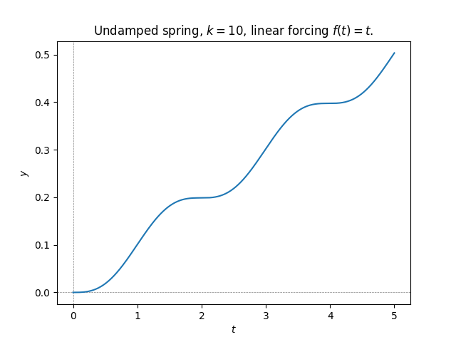
Since there is no damping the continuously increasing force causes the spring to extend indefinitely (of course for an actual physical spring this will cause the spring to break and the model to break down after some amount of time).
\(\text{ }\) Oscillating external force. Consider now a sinusoidal periodic external force \[f(t)=\cos(\theta t)\] for \(\theta>0.\) To find a particular solution we make the ansatz \[y(t)=a\cos(\theta t)+b\sin(\theta t).\] For this ansatz \[y'(t)=-a\theta\sin(\theta t)+b\theta\cos(\theta t),\] and \[y''(t)=-a\theta^{2}\sin(\theta t)-b\theta^{2}\cos(\theta t),\] and so \[y''(t)+ky=a(k-\theta^{2})\cos(t\theta)+b(k-\theta^{2})\sin(t\theta).\] This equals \(\cos(t\theta)\) identically if \[\begin{array}{l} a(k-\theta^{2})=1,\\ b(k-\theta^{2})=0. \end{array}\] Note that this system of scalar equations has a solution only if \(\theta\ne\sqrt{k},\) and then the solution is \[a=\frac{1}{k-\theta^{2}}\quad\text{ and }\quad b=0,\] giving the particular solution \[y_{p}(t)=\frac{1}{k-\theta^{2}}\cos(\theta t).\] As before, to solve the IVP ([eq:ch9_forced_spring_IVP]) we need to add a solution \(y_{h}(t)\) of the homogeneous equation \[y''+ky=0,\] which have the form \[y_{h}(t)=\alpha\cos(t\sqrt{k})+\beta\sin(t\sqrt{k}).\] Thus the general solution to the non-homogeneous ODE ([eq:ch9_forced_undamped_spring_ODE]) is \[y(t)=\alpha\cos(t\sqrt{k})+\beta\sin(t\sqrt{k})+\frac{1}{k-\theta^{2}}\cos(\theta t).\] For this \(y(t)\) \[y'(t)=-\sqrt{k}\alpha\sin(\sqrt{k}\alpha)+\sqrt{k}\beta\cos(\sqrt{k}\beta)-\frac{1}{k-\theta^{2}}\sin(\theta t).\] Thus \(y(0)=\alpha+\frac{1}{k-\theta^{2}}\) and \(y'(0)=\sqrt{k}\beta,\) so the IVP is solved if \[\alpha+\frac{1}{k-\theta^{2}}=0,\sqrt{k}\beta=0\iff\alpha-\frac{1}{k-\theta^{2}},\beta=-0.\] Thus the solution is \[y(t)=\frac{1}{k-\theta^{2}}\left(\cos(\theta t)-\cos(\sqrt{k}t)\right),\] shown in the next figure.
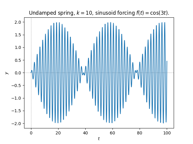
The combination of two sinusoids of different frequencies lead to a modulated sinusoid. Since the external force is not always acting in the same direction, it sometimes accelerates and sometimes decelerates the mass, and the extension of the spring stays bounded for all \(t\ge0.\)
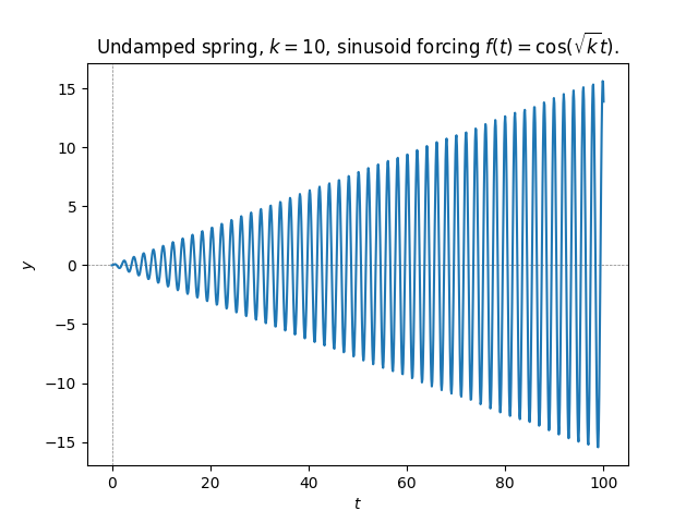
\(\text{ }\) Resonant case. Let us now consider the case \(f(\theta)=\cos(\theta t)\) with \(\theta=\sqrt{k}.\) The computation above failed to solve the IVP ([eq:ch9_forced_spring_IVP]) in this case. This was because our ansatz for a particular solution was not successful when \(\theta=\sqrt{k}.\) Indeed our ansatz was a combination of \(\cos(\theta t)\) and \(\sin(\theta t),\) and when \(\theta=\sqrt{k}\) these are already solutions to the homogeneous equation, so they cannot yield solutions to the non-homogeneous equation.
This situation is similar to the case of a \(k\)-th order autonomous homogeneous linear equation when the characteristic equation has a repeated root: if \(r_{1}\ne r_{2}\) are distinct roots, then \(e^{r_{i}t},i=1,2\) yield two different solutions, but if \(r_{1}=r_{2}\) we only get one solution from these two eigenvalues. It turned out that another distinct solution could be obtained by multiplying \(e^{rt}\) by \(t.\) Inspired by this, we try the ansatz \[y(t)=at\cos(\sqrt{k}t)+bt\sin(\sqrt{k}t).\] For this \(y\) \[y'(t)=\cos(\sqrt{k}t)\left(a+\sqrt{k}tu\right)+\sin(\sqrt{k}t)\left(u-\sqrt{k}\alpha t\right),\] and \[y''(t)=\cos(\sqrt{k}t)\left(2\sqrt{k}u-kat\right)+\sin(\sqrt{k}t)\left(-2a\sqrt{k}-ktb\right).\] This gives \[y''(t)+ky=2b\sqrt{k}\cos(\sqrt{k}t)-2a\sqrt{k}\sin(\sqrt{k}t).\] This equals \(\cos(\sqrt{k}t)\) identically if \[2b\sqrt{k}=1\text{ and }2a\sqrt{k}=0\iff a=0,b=\frac{1}{2\sqrt{k}}.\] Thus we have successfully found the particular solution \[y_{p}(t)=\frac{t}{2\sqrt{k}}\sin(\sqrt{k}t).\] Adding the general solution of the homogeneous equation yields \[y(t)=\alpha\cos(t\sqrt{k})+\beta\sin(t\sqrt{k})+\frac{t}{2\sqrt{k}}\sin(\sqrt{k}t).\] For this \(y(t)\) we have \[y'(t)=\left(\frac{1}{2\sqrt{k}}-\alpha\sqrt{k}\right)\sin(\sqrt{k}t)+\left(\beta\sqrt{k}+\frac{t}{2}\right)\cos(\sqrt{k}t),\] and so \(y(0)=\alpha\) and \(y'(0)=\beta\sqrt{k},\) so the IVP is solved if \[\alpha=0\quad\quad\beta=0.\] Thus the solution to the IVP ([eq:ch9_forced_spring_IVP]) is \[y(t)=\frac{t}{2\sqrt{k}}\sin(\sqrt{k}t).\] Coincidentally, our particular solution already solves the IVP in this case (this is just a fluke with no particular significance). Here is a plot of the solution.
 s
s
The spring oscillates at frequency \(\sqrt{k},\) as it does without forcing, but here the amplitude grows without bounds. This is because the frequency of the external force is just right so as to minimize the amount deceleration the force causes, and maximize the acceleration (i.e. the force further extends the spring when its momentum is already extending it, and compresses the spring when the momentum is already compressing it). This phenomenon is called resonance. Even complex physical systems generally have such a “resonant frequency”, whereby a small periodic external force with this frequency can cause a very large oscillation of the whole system. Resonance can cause bridges to collapse if the wind or traffic happens to cause oscillation at precisely the resonant frequency, as happened in 1940 in Tacoma, USA and was caught on film.
9 Numerical solution I:
first steps
This chapter is heavily inspired by Chapter I.1 of A First Course in the Numerical Analysis of Differential Equations by Arieh Iserles.
9.1 Euler’s method
The simplest algorithm for solving ODEs numerically is Euler’s method. It is the one we mentioned in the introduction in Section 1.4. It is also the starting point from which we develop more sophisticated methods.
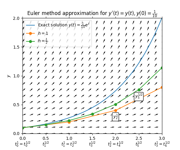
\(\text{ }\) Heuristic derivation Let \[\dot{y}=F(t,y),\quad\quad t\in I,\quad\quad y(t_{0})=y_{0},\tag{9.1}\] be an IVP. Any solution to the IVP must satisfy \[y(t)=y(t_{0})+\int_{t_{0}}^{t}F(s,y(s))ds,\] for all \(t\in I.\) Euler’s method is motivated by the approximation \[\int_{t_{0}}^{t}F(s,y(s))ds\approx(t-t_{0})F(t_{0},y(t_{0})).\] For continuous \(F\) and \(y\) this is a reasonable approximation if \(t-t_{0}\) is sufficiently small. So letting \(t_{1}=t_{0}+h\) for a small \(h,\) we define \[y_{1}=y_{0}+hF(t_{0},y_{0}),\] as the approximation of \(y(t_{1}).\) To get an approximation for larger values of \(t\) one iterates this, letting \(t_{2}=t_{1}+h=t_{0}+2h\) and approximating \(y(t_{2})\) by \[y_{2}=y_{1}+hF(t_{0},y_{0})=y_{0}+hF(t_{0},y_{0})+hF(t_{1},y_{1}).\] Continuing like this one ends up with a grid of “times” \(t_{n}\) with spacing \(h\) given by \[t_{n+1}=t_{n}+h,n=0,1,2,\ldots,\quad\text{so that }t_{n}=t_{0}+nh,\] and recursively defined approximations \[y_{n+1}=y_{n}+hF(t_{n},y_{n}),n=0,1,\ldots.\] For small \(h\) one can hope that the solution \(y(t)\) to the IVP satisfies \[y(t_{n})\approx y_{n}.\] When the step-size being used is not unambiguous from the context we indicate it as a super-script, writing e.g. \[y_{n+1}^{h}=y_{n}^{h}+hF(t_{n}^{h},y_{n}^{h}).\] The next plot shows the result of applying Euler’s method to the ODE \(y'=y\) for two different step-sizes.
\(\text{ }\) Formal definition Let us state the above in a formal definition. Note that the derivations above work for \(\mathbb{R}^{d}\)- and \(\mathbb{C}^{d}\)-valued ODEs for any \(d\ge1.\)
Let \(d\ge1,\) and \(V=\mathbb{R}^{d}\) or \(V=\mathbb{C}^{d}.\) Let \(t_{0},t_{\max}\in\mathbb{R},t_{0}<t_{\max}\) and \(I=[t_{0},t_{\max}).\) Let \(F:I\times V\to V\) and \(y_{0}\in V.\) Let \(h>0.\) Consider the IVP \[\dot{y}(t)=F(t,y(t)),\quad\quad t\in I,\quad\quad y(t_{0})=y_{0}.\tag{9.3}\] Let \(t_{n}=t_{0}+nh,n\ge0\) and define recursively \[y_{n+1}=y_{n}+hF(t_{n},y_{n}),\tag{9.4}\] for all \(n\ge0\) such that \(t_{n}<t_{\max}\) . The sequence \(y_{n},n\ge0\) is the approximation of the Euler method.
\(\text{ }\) Implementation The Euler method is easy to implement on a computer. Here is an implementation in Python.
def euler( F, h, t0, tmax, y0 ):
  """
  Solves an initial value problem (IVP) using Euler's method.
  Parameters:
  F (function F(t,y)): the right-hand side of the ODE, y' = F(t, y).
  h (float): The step size.
  t0 (float): The initial value of t.
  tmax (float): The final value of t.
  y0 (float): The initial value of y.
  Returns:
  th (list): A list of t values at each step.
  yh (list): A list of y values at each step.
  """
  th = [t0]
  yh = [y0]
  while th[-1]<tmax:
    th.append( th[-1] + h )
    yh.append( yh[-1] + h*F( th[-1], yh[-1] ) )
  return th, yh

th, yh = euler( lambda t, y: y**2, 0.1, 0, 1, 1 )
print(th)
print(yh)
\(\text{ }\) Analyzing the error Our next task is to study the error of the algorithm, and how it depends on \(h.\) At the very least the error should tend to zero for \(h\downarrow0.\) We are also interested in how fast the error decays as \(h\downarrow0.\)
\(\text{ }\) Error of Riemann sum First, consider the error in the approximation \[\int_{t_{0}}^{t_{1}}f(t)dt\approx(t_{1}-t_{0})f(t_{0})\tag{9.5}\] of an definite integral of an arbitrary function \(f.\) If \(f\) is differentiable with bounded derivative on \([t_{0},t_{\max}],\) then by Taylor’s theorem there exists for each \(t\in[t_{0},t_{1}]\) an \(s\in[t_{0},t]\) such that \(f(t)=f(t_{0})+(t-t_{0})f'(s).\) This implies that \[\left|f(t)-f(t_{0})\right|\le(t-t_{0})K\le Kh\quad\quad\text{for}\quad\quad K=\sup_{s\in[t_{0},t_{\max}]}\left|f'(s)\right|.\] Using this to bound the error in ([eq:ch9_riemann_one_summand_approx]) we obtain \[\left|\int_{t_{0}}^{t_{1}}f(t)dt-hf(t_{0})\right|=\left|\int_{t_{0}}^{t_{1}}(f(t)-f(t_{0}))dt\right|\le\int_{t_{0}}^{t_{1}}\left|f(t)-f(t_{0})\right|dt\le Kh^{2}.\tag{9.6}\] Thus the error converges to zero as \(h\downarrow0,\) at a quadratic rate.
This is the basic step of bounding the error when approximating a definite integral \(\int_{t_{0}}^{t_{\max}}f(t)dt\) by the (left) Riemann sum \(\sum_{0\le n\le\frac{t_{\max}}{h}}hf(t_{n}).\) For simplicity, assume that \(t_{\max}=t_{0}+Nh\) for a positive integer \(N,\) in which case using ([eq:ch9_def_int_riemann_err_one_step]) on each interval \([t_{n},t_{n+1}]\) (i.e. with this interval in place of \([t_{0},t_{1}]\)) one obtains \[\begin{array}{ccl} \left|\int_{t_{0}}^{t_{\max}}f(t)dt-{\displaystyle \sum_{0\le n\le N-1}}hf(t_{n})\right| & = & \left|{\displaystyle \sum_{0\le n\le N-1}}\left(\int_{t_{n}}^{t_{n+1}}f(t)dt-hf(t_{n})\right)\right|\\ & \le & {\displaystyle \sum_{0\le n\le N-1}}\left|\int_{t_{n}}^{t_{n+1}}f(t)dt-hf(t_{n})\right|\\ & \le & Kh^{2}N\\ & = & K(t_{\max}-t_{0})h. \end{array}\tag{9.7}\] This standard estimate shows that the (left) Riemann sum has an error converging to zero as \(h\downarrow0,\) linearly in \(h.\)
\(\text{ }\) Error of Euler method Turning to Euler’s method, we start by considering the error in one step of the method, that is \[e_{1}=y_{1}-y(t_{1}),\] where \(y\) is the solution to the IVP ([eq:ch9_euler_method_def_IVP]). By ([eq:ch9_euler_method_def_one_step]) and the identity \(y(t_{1})=y(t_{0})+\int_{t_{0}}^{t_{1}}F(t,y(t))dt\) this equals \[e_{1}=hF(t_{0},y_{0})-\int_{t_{0}}^{t_{1}}F(t,y(t))dt.\tag{9.8}\] By ([eq:ch9_def_int_riemann_err_one_step]) with \(f(t)=F(t,y(t))\) this is bounded above by \[\left|e_{1}\right|\le Kh^{2}\quad\quad\quad\text{for }\quad\quad\quad K=\sup_{s\in[t_{0},t_{\max}]}\left|\frac{d}{dt}F(t,y(t))\right|,\] provided \(t\to F(t,y(t))\) is differentiable. This will be the case if \(F(t,y)\) is differentiable as a function of \((t,y),\) since \(y\) a solution to the ODE and therefore necessarily differentiable. Whenever a numerical method has an error in one step of at most \(ch^{p+1}\) for some \(c>0,\) we call it a \(p\)-th order method (see formal definition below). The Euler method is thus a first order method.
Next we consider the error in the second step: \[e_{2}=y_{2}-y(t_{2}).\tag{9.9}\] By ([eq:ch9_euler_method_def_one_step]) and the identity \(y(t_{2})=y(t_{1})+\int_{t_{1}}^{t_{2}}F(t,y(t))dt\) this equals \[e_{1}+hF(t_{1},y_{1})-\int_{t_{1}}^{t_{2}}F(t,y(t))dt,\] so \[\left|e_{2}\right|\le\left|e_{1}\right|+\left|hF(t_{1},y_{1})-\int_{t_{1}}^{t_{2}}F(t,y(t))dt\right|.\] The second term is not quite like ([eq:ch9_euler_error_analysis_e1]), since \(y_{1}\ne y(t_{1}).\) Thus we first use that \[\left|F(t_{1},y_{1})-F(t_{1},y(t_{1}))\right|\le L\left|e_{1}\right|,\] where \(L\) is the Lipschitz constant of \(F\) as function of \((t,y)\) (we assume it is Lipschitz). By the triangle inequality \[\left|hF(t_{1},y_{1})-\int_{t_{1}}^{t_{2}}F(t,y(t))dt\right|\le Lh\left|e_{1}\right|+\left|hF(t_{1},y(t_{1}))-\int_{t_{1}}^{t_{2}}F(t,y(t))dt\right|.\] Now we can use ([eq:ch9_def_int_riemann_err_one_step]) with \(f(t)=F(t,y(t))\) to bound the last term by \(Kh^{2},\) and we arrive at the upper bound \[\left|e_{2}\right|\le\left(1+Lh\right)\left|e_{1}\right|+Kh^{2}.\] The same computation shows that \[\left|e_{n+1}\right|\le\left(1+Lh\right)\left|e_{n}\right|+Kh^{2},n\ge0.\] Below we will see that this implies that \[\left|e_{n}\right|\le K\frac{e^{Lt_{\max}}-1}{L}h\tag{9.10}\] for all \(0\le n\le\frac{t_{\max}}{h}.\) Thus the global error of Euler’s method decays to zero as \(h\downarrow0.\) We say that the method is convergent (see formal definition and proof below). Furthermore the error decays linearly in \(h.\)
\(\text{ }\) Formal definitions Let us now introduce some formal definitions. Firstly, we define the following general class of time-stepping methods.
A time-stepping method is a sequence of functions \[Y_{n}(F,h,t_{0},y_{0},y_{1},\ldots,y_{n})\quad\quad n=0,1,2,\ldots\] that take as input an \(F:[t_{0},t_{\max}]\times V\to V,\) where \(t_{0}\in\mathbb{R},t_{\max}\in\mathbb{R},t_{0}<t_{\max}\) and \(V=\mathbb{R}^{d}\) or \(V=\mathbb{C}^{d},\) and a step-size \(h>0,\) and outputs an element of \(V.\)
The output of the time-stepping method is the sequence \[y_{n+1}=Y_{n}(F,h,t_{0},y_{0},\ldots,y_{n})\quad\quad0\le n\le\frac{t_{\max}-t_{0}}{h}.\] If the IVP \[\dot{y}(t)=F(t,y(t)),\quad\quad t\in I,\quad\quad y(t_{0})=y_{0},\tag{9.11}\] has a unique solution \(y,\) then the errors of the method is \[e_{n}=y_{n}-y(t_{n})\quad\quad0\le n\le\frac{t_{\max}-t_{0}}{h}.\tag{9.12}\] The global error over the whole interval \([t_{0},t_{\max}]\) is \[\max_{0\le n\le\frac{t_{\max}-t_{0}}{h}}\left|e_{n}\right|.\]
Let \(d\ge1,\) and \(V=\mathbb{R}^{d}\) or \(V=\mathbb{C}^{d}.\) Let \(t_{0},t_{\max}\in\mathbb{R},t_{0}<t_{\max}\) and \(I=[t_{0},t_{\max}).\) Let \(F:I\times V\to V\) and \(y_{0}\in V.\) Let \(h>0.\) Consider the IVP \[\dot{y}(t)=F(t,y(t)),\quad\quad t\in I,\quad\quad y(t_{0})=y_{0}.\tag{9.3}\] Let \(t_{n}=t_{0}+nh,n\ge0\) and define recursively \[y_{n+1}=y_{n}+hF(t_{n},y_{n}),\tag{9.4}\] for all \(n\ge0\) such that \(t_{n}<t_{\max}\) . The sequence \(y_{n},n\ge0\) is the approximation of the Euler method.
A time-stepping method is a sequence of functions \[Y_{n}(F,h,t_{0},y_{0},y_{1},\ldots,y_{n})\quad\quad n=0,1,2,\ldots\] that take as input an \(F:[t_{0},t_{\max}]\times V\to V,\) where \(t_{0}\in\mathbb{R},t_{\max}\in\mathbb{R},t_{0}<t_{\max}\) and \(V=\mathbb{R}^{d}\) or \(V=\mathbb{C}^{d},\) and a step-size \(h>0,\) and outputs an element of \(V.\)
The output of the time-stepping method is the sequence \[y_{n+1}=Y_{n}(F,h,t_{0},y_{0},\ldots,y_{n})\quad\quad0\le n\le\frac{t_{\max}-t_{0}}{h}.\] If the IVP \[\dot{y}(t)=F(t,y(t)),\quad\quad t\in I,\quad\quad y(t_{0})=y_{0},\tag{9.11}\] has a unique solution \(y,\) then the errors of the method is \[e_{n}=y_{n}-y(t_{n})\quad\quad0\le n\le\frac{t_{\max}-t_{0}}{h}.\tag{9.12}\] The global error over the whole interval \([t_{0},t_{\max}]\) is \[\max_{0\le n\le\frac{t_{\max}-t_{0}}{h}}\left|e_{n}\right|.\]
1) Note that ([eq:ch9_time_stepping_method_order_local_err]) is the error the method does in approximating \(y(t_{n+1}),\) when it has access to the exact values of \(y(t_{m})\) for \(m\le n.\) It is thus a local error.
2) Recall that a function \(f:\mathbb{R}^{d}\to\mathbb{R}\) or \(f:\mathbb{C}^{d}\to\mathbb{C}\) is analytic if at each point of its domain it has a power series with a positive radius of convergence. A function \(f:\mathbb{R}^{d}\to\mathbb{R}^{d'}\) or \(f:\mathbb{C}^{d}\to\mathbb{C}^{d'}\) is analytic if each of its components are analytic functions.
Concretely, for a function \(f:\mathbb{R}^{d}\to\mathbb{R}\) or \(f:\mathbb{C}^{d}\to\mathbb{C}\) this means that for each \(x\) there exists an \(r>0\) and constants \(a_{0},a_{1},\ldots\) such that \[f(z)=\sum_{n\ge0}a_{n}(z-x)^{n}\text{ if }|z-x|<r.\] A function that is analytic is also infinitely differentiable, and for each \(x\) the \(a_{n}\) above are given by \[a_{n}=\frac{f^{(n)}(x)}{n!}.\] For a function \(f:\mathbb{R}^{d}\to\mathbb{R}\) or \(f:\mathbb{C}^{d}\to\mathbb{C}\) it means that there are constants \(a_{n_{1},\ldots,n_{d}}\) such that \[f(z)=\sum_{n_{1},\ldots,n_{d}\ge0}a_{n_{1},\ldots,n_{d}}\prod_{i=1}^{d}(z_{i}-x_{i})^{n_{i}}\text{ if }|z-x|<r.\] Such an \(f\) is infinitely differentiable, and the expansion can be written as \[f(z)=\sum_{n_{1},\ldots,n_{d}\ge0}\frac{1}{n_{1}!\ldots n_{d}!}\frac{\partial f}{\partial x_{n_{1}}\ldots\partial x_{n_{d}}}(z)\prod_{i=1}^{d}(z_{i}-x_{i})^{n_{i}}\text{ if }|z-x|<r.\]
We use the analyticity hypothesis in the definition above to simplify subsequent proofs. A more general treatment would use a Lipschitz assumption instead.
We record without proof the following result, which states that if the \(F\) of an ODE is analytic, then its solutions are analytic.
Let \(d\ge1,\) and \(V=\mathbb{R}^{d}\) or \(V=\mathbb{C}^{d}.\) Let \(t_{0},t_{\max}\in\mathbb{R},t_{0}<t_{\max}\) and \(I=[t_{0},t_{\max}].\) Let \(F:I\times V\to V\) and \(y_{0}\in V.\) Let \(h>0.\) Assume that \(F\) is analytic. If the IVP \[\dot{y}(t)=F(t,y(t)),\quad\quad t\in I,\quad\quad y(t_{0})=y_{0},\tag{9.16}\] has a solution \(y:I\to V,\) then \(y\) is analytic.
Next we record formally that Euler’s method is of order \(p=1.\)
Let \(d\ge1,\) and \(V=\mathbb{R}^{d}\) or \(V=\mathbb{C}^{d}.\) Let \(t_{0},t_{\max}\in\mathbb{R},t_{0}<t_{\max}\) and \(I=[t_{0},t_{\max}).\) Let \(F:I\times V\to V\) and \(y_{0}\in V.\) Let \(h>0.\) Consider the IVP \[\dot{y}(t)=F(t,y(t)),\quad\quad t\in I,\quad\quad y(t_{0})=y_{0}.\tag{9.3}\] Let \(t_{n}=t_{0}+nh,n\ge0\) and define recursively \[y_{n+1}=y_{n}+hF(t_{n},y_{n}),\tag{9.4}\] for all \(n\ge0\) such that \(t_{n}<t_{\max}\) . The sequence \(y_{n},n\ge0\) is the approximation of the Euler method.
Proof. For this method the l.h.s. of ([eq:ch9_time_stepping_method_order_local_err]) equals \[\left|y(t_{n+1})-hF(t_{n},y(t_{n}))\right|,\] where \(y\) is the unique solution to ([eq:ch9_numerical_time_stepping_def_IVP]) on \([t_{0},t_{n+1}].\) Since \(F\) is analytic \(y\) is also analytic, and so is \(t\to F(t,y(t)).\) In particular \(t\to F(t,y(t))\) is continuously differentiable, so using Taylor’s theorem as in ([eq:ch9_riemann_one_summand_approx])-([eq:ch9_def_int_riemann_err_one_step]) we obtain \[\left|y(t_{n+1})-hF(t_{n},y(t_{n}))\right|\le Kh^{2}\tag{9.17}\] where \[K=\sup_{t\in[t_{n},t_{n+1}]}\left|\frac{d}{dt}F(t,y(t))\right|\] is finite because \(t\to\frac{d}{dt}F(t,y(t))\) is a continuous function on the compact interval \([t_{n},t_{n+1}].\)
A time-stepping method is a sequence of functions \[Y_{n}(F,h,t_{0},y_{0},y_{1},\ldots,y_{n})\quad\quad n=0,1,2,\ldots\] that take as input an \(F:[t_{0},t_{\max}]\times V\to V,\) where \(t_{0}\in\mathbb{R},t_{\max}\in\mathbb{R},t_{0}<t_{\max}\) and \(V=\mathbb{R}^{d}\) or \(V=\mathbb{C}^{d},\) and a step-size \(h>0,\) and outputs an element of \(V.\)
The output of the time-stepping method is the sequence \[y_{n+1}=Y_{n}(F,h,t_{0},y_{0},\ldots,y_{n})\quad\quad0\le n\le\frac{t_{\max}-t_{0}}{h}.\] If the IVP \[\dot{y}(t)=F(t,y(t)),\quad\quad t\in I,\quad\quad y(t_{0})=y_{0},\tag{9.11}\] has a unique solution \(y,\) then the errors of the method is \[e_{n}=y_{n}-y(t_{n})\quad\quad0\le n\le\frac{t_{\max}-t_{0}}{h}.\tag{9.12}\] The global error over the whole interval \([t_{0},t_{\max}]\) is \[\max_{0\le n\le\frac{t_{\max}-t_{0}}{h}}\left|e_{n}\right|.\]
Let \(d\ge1,\) and \(V=\mathbb{R}^{d}\) or \(V=\mathbb{C}^{d}.\) Let \(t_{0},t_{\max}\in\mathbb{R},t_{0}<t_{\max}\) and \(I=[t_{0},t_{\max}).\) Let \(F:I\times V\to V\) and \(y_{0}\in V.\) Let \(h>0.\) Consider the IVP \[\dot{y}(t)=F(t,y(t)),\quad\quad t\in I,\quad\quad y(t_{0})=y_{0}.\tag{9.3}\] Let \(t_{n}=t_{0}+nh,n\ge0\) and define recursively \[y_{n+1}=y_{n}+hF(t_{n},y_{n}),\tag{9.4}\] for all \(n\ge0\) such that \(t_{n}<t_{\max}\) . The sequence \(y_{n},n\ge0\) is the approximation of the Euler method.
Proof. To argue as in ([eq:ch9_euler_error_analysis_e2])-([eq:ch9_euler_error_analysis_global_err_final]) we need \(F\) to be Lipschitz, which may not be the case on whole domain \(V,\) even if \(F\) is assumed to be analytic (e.g. \(f(x)=x^{2}\) is analytic but not Lipschitz on \(\mathbb{R}\)). To overcome this technical point we need to argue that we can restrict attention to a compact subset of \(V.\) To this end, note that if \(F\) is analytic, then so is \(y\) and \(t\to F(t,y(t)).\) Since \(y\) is continuous \(\sup_{t\in[t_{0},t_{\max}]}|y(t)|<\infty.\) Furthermore, let \[M_{n}=\sup_{t\in I,y:|y|\le\left|y_{n}^{1}\right|}\left|F(t,y)\right|,\] for the result \(y_{n}^{1}\) of the Euler method with \(h=1,\) which must be a finite quantity since for all \(n\) since \(F\) is continuous and the supremum is always taken over a compact set. We then have that \[\left|y_{n}^{1}\right|\le M_{1}+M_{2}+\ldots+M_{n}\text{ for all }n,\] and for \(h\in(0,1]\) \[|y_{n}^{h}|\le M_{1}+hM_{2}+\ldots+hM_{n}\le M_{1}+\ldots+M_{n}\text{ for all }n.\] Thus \[\sup_{h\in(0,1]}\max_{0\le n\le t_{\max}}|y_{n}^{h}|<\infty,\] so \[A=\left\{ z\in V:\left|z\right|\le\max\left(\sup_{h\in(0,1]}\max_{0\le n\le t_{\max}}|y_{n}^{h}|,\sup_{t\in[t_{0},t_{\max}]}|y(t)|\right)\right\}\] is a compact convex set such that \(y_{n}^{h}\in A\) for all \(h\in(0,1],\) \(0\le n\le\frac{t_{\max}}{h}\) and \(y(t)\in A\) for all \(t\in I.\) Now let \[L=\sup_{t\in I,y\in A}\left|\nabla F(t,y)\right|,\] be the Lipschitz constant constant of \(F\) on \(A,\) which must be finite since \(I\times A\) is compact. We can now argue as in ([eq:ch9_euler_error_analysis_e2])-([eq:ch9_euler_error_analysis_global_err_final]).
Dropping the superscript \(h\) we have for \(h\in(0,1]\) that \[\begin{array}{ccl} |e_{n+1}| & \le & |e_{n}|+\left|\int_{t_{n}}^{t_{n+1}}F(t,y(t))dt-hF(t_{n},y_{n})\right|\\ & \le & |e_{n}|+h\left|F(t_{n},y_{n})-F(t_{n},y(t_{n}))\right|+\left|\int_{t_{n}}^{t_{n+1}}F(t,y(t))dt-hF(t_{n},y(t_{n}))\right|\\ & \le & |e_{n}|+hL|e_{n}|+Kh^{2}, \end{array}\] for all \(0\le n\le\frac{t_{\max}}{h},\) where \[K=\sup_{t\in I}\left|\frac{d}{dt}F(t,y(t))\right|,\] which must be finite by continuity of \(t\to F(t,y(t))\) and the compactness of \(I.\) The last step uses ([eq:ch9_def_int_riemann_err_one_step]). By induction on \(n\) it follows that \[|e_{n}|\le K\sum_{m=0}^{n-1}(1+hL)^{m}h^{2}\text{ for all }0\le n\le\frac{t_{\max}}{h}.\] Note that \[\sum_{m=0}^{n-1}(1+hL)^{m}=\frac{(1+hL)^{n}-1}{hL},\] and using the inequality \(1+x\le e^{x},x\ge0\) and \(n\le\frac{t_{\max}}{h}\) \[(1+hL)^{n}\le e^{hLn}\le e^{Lt_{\max}}.\] Therefore \[|e_{n}|\le\frac{K}{L}e^{Lt_{\max}}h\text{ for all }0\le n\le\frac{t_{\max}}{h}.\tag{9.20}\] Thus \[\max_{0\le n\le\frac{t_{\max}}{h}}|e_{n}|\le\frac{K}{L}e^{Lt_{\max}}h\downarrow0\quad\quad\text{ as }\quad\quad h\downarrow0,\] so the method is convergent.
9.2 Euler’s method for higher order equations
Suppose we want to numerically solve a second order IVP \[y''=F(t,y',y),\quad\quad y(t_{0})=y_{0}^{0},y'(t_{0})=y_{0}^{1}.\tag{9.21}\] A natural approach would be to compute two sequences \[y_{n}^{0},y_{n}^{1},\] where \(y_{n}^{0}\) approximates \(y(t_{n})\) and \(y_{n}^{1}\) approximates \(y'(t_{n}).\) Since \[y(t_{n+1})=y(t_{n})+\int_{t_{n}}^{t_{n+1}}y_{n}'(t)dt,\] and \[y'(t_{n+1})=y'(t_{n})+\int_{t_{n}}^{t_{n+1}}y_{n}''(t)dt=y'(t_{n})+\int_{t_{n}}^{t_{n+1}}F(t,y'(t),y(t))dt\] the natural update rule in the spirit of Euler’s method is \[\begin{array}{ccl} y_{n+1}^{0} & = & y_{n}^{0}+hy_{n}^{1},\\ y_{n+1}^{1} & = & y_{n}^{1}+hF(t_{n},y_{n}^{1},y_{n}^{0}). \end{array}\tag{9.22}\]
Let \(d\ge1,\) and \(V=\mathbb{R}^{d}\) or \(V=\mathbb{C}^{d}.\) Let \(t_{0},t_{\max}\in\mathbb{R},t_{0}<t_{\max}\) and \(I=[t_{0},t_{\max}).\) Let \(F:I\times V\to V\) and \(y_{0}\in V.\) Let \(h>0.\) Consider the IVP \[\dot{y}(t)=F(t,y(t)),\quad\quad t\in I,\quad\quad y(t_{0})=y_{0}.\tag{9.3}\] Let \(t_{n}=t_{0}+nh,n\ge0\) and define recursively \[y_{n+1}=y_{n}+hF(t_{n},y_{n}),\tag{9.4}\] for all \(n\ge0\) such that \(t_{n}<t_{\max}\) . The sequence \(y_{n},n\ge0\) is the approximation of the Euler method.
For a general \(k\)-th order ODE \[y^{(k)}=F(t,y^{(k-1)},\ldots,y),\quad\quad y^{(l)}(t_{0})=y_{0}^{l},l=0,\ldots,k-1,\] either approach yields the same update rule for the sequence of approximations \((y_{n}^{k-1},y_{n}^{k-2},\ldots,y_{n}^{0})\): \[\begin{array}{ccl} y_{n+1}^{l} & = & y_{n}^{l}+hy_{n}^{l+1}\text{ for }l=0,\ldots,k-2,\\ y_{n+1}^{k-1} & = & y_{n}^{k-1}+hF(t_{n},y_{n}^{k-1},\ldots,y_{n}^{0}). \end{array}\]