The problem \[\text{minimize }\,\:(x-y)^{2}-x-y\,\:\text{ subject to }\,\:\left(x-\frac{1}{4}\right)^{2}+2y^{2}=\frac{1}{2}\tag{3.1}\] is a constrained optimization problem, because to solve it one must optimize the objective function \(f(x)\) not over all \(x,\) but only over \(x\) that satisfy the constraint \(\left(x-\frac{1}{4}\right)^{2}+2y^{2}=\frac{1}{2}.\) Such problems are common in many applications. For instance, imagine we plan to build a shed with dimensions \(x\times y\times z\) meters, and the cost of the materials is \(R\) CHF/\(m^{2}\) for the roof, \(W\) CHF/\(m^{2}\) for the walls and \(F\) CHF/\(m^{2}\) for the floor. Then for given dimensions \(x,y,z\) the total cost is \((F+R)xy+W(2xz+2yz).\) The largest volume shed we can build with a budgetary constraint of \(4000\) CHF is the solution of constrained optimization problem \[\text{maximize }\,xyz\:\text{ subject to }\begin{cases} (F+R)xy+W(2xz+2yz)\le4000,\\ x\ge0,y\ge0,z\ge0. \end{cases}\]
The general form of a constrained optimization problem of the type ([eq:ch2_const_opt_first_ex]) is \[\text{minimize }\,\:f(x)\,\:\text{ subject to }\,\:h(x)=0,\tag{3.2}\] for an objective function \(f:\mathbb{R}^{d}\to\mathbb{R}\) and a constraint function \({h:\mathbb{R}^{d}\to\mathbb{R}}\) (this standard form of course also covers constrained maximization). Solving the critical point equation \[\nabla f(x)=0\tag{3.3}\] of the objective function is not helpful in finding optima of the constrained optimization problem ([eq:ch2_const_opt_one_eq_const_general_form]), since a critical point of \(f\) will in general not satisfy the constraint. There is however a different but related equation that can be solved to find optima for constrained problems.
3.1 Lagrange multipliers
It turns out that the optimization problem ([eq:ch2_const_opt_one_eq_const_general_form]) with the constraint \({h(x)=0}\) has a kind of “critical point equation” which reads \[\nabla f(x)=\lambda\nabla h(x),\tag{3.4}\] where \(\lambda\) is an additional variable to be solved for, called a Lagrange multiplier. Below you will see how the method of Lagrange multipliers uses this equation in practice. But first, let us heuristically derive the equation ([eq:ch2_lagrange_mult_first_appearence]) using geometrical intuition.
For any constraint \(h(x)=0,\) let \(I_{h}\) denote the subset of \(\mathbb{R}^{d}\) of points that satisfy the constraint, i.e. \(I_{h}=\{x\in\mathbb{R}^{d}:h(x)=0\}.\) Consider \(f|_{I_{h}},\) the objective function \(f\) restricted to this smaller domain. We will argue that if \(x\in I_{h}\) is a local minimum of \(f|_{I_{h}},\) then it satisfies ([eq:ch2_lagrange_mult_first_appearence]) for some \(\lambda\) (at least usually). Cf. Lemma 2.6, which proves that if \(x\in\mathbb{R}^{d}\) is a local minimum of \(f\) (without constraint/restriction), then it satisfies ([eq:ch3_unconstrained_crit_point_eq]). Note that being a local minimum of \(f|_{I_{h}}\) is a weaker condition than being a local minimum of \(f,\) since the latter condition requires the existence of an \(\varepsilon>0\) s.t. \(f(x)\le f(y)\) whenever \(y\in\mathbb{R}^{d}\) and \(|x-y|\le\varepsilon,\) while the former condition requires \(f(x)\le f(y)\) only whenever \(y\in I_{h}\) and \(|x-y|\le\varepsilon.\)
Gradients and descent directions
For a differentiable function \({f:\mathbb{R}^{d}\to\mathbb{R}},\) the gradient \(\nabla f(x)\) at a point \(x\) is the direction of fastest ascent (increase) of \(f.\) That is, if one were to move slightly away from \(x\) in some direction, the value of \(f\) will increase the fastest if that direction is \(\nabla f(x),\) provided \(\nabla f(x)\ne0.\) The negative gradient \(-\nabla f(x)\) is the direction of fastest descent (decrease), provided \(\nabla f(x)\ne0.\)
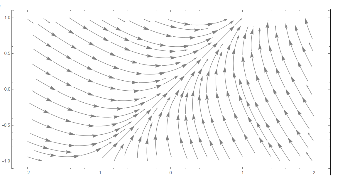
If \(\nabla f(x)\ne0\) for a given \(x,\) then moving from \(x\) to a sufficiently close point \(x'\) in the direction of \(-\nabla f(x)\) is guaranteed to yield a strictly lower value of \(f.\) This is in fact true for any direction \(v\) such that the directional derivative \(\partial_{v}f(x)\) is negative. Recall that the directional derivative is given by \[\partial_{v}f(x)=\nabla f(x)\cdot v,\] (for any unit vector \(v,\) i.e. \(v\in\mathbb{R}^{d}\) s.t. \(|v|=1\)). Thus moving a small enough distance in any direction \(v\) with a negative inner product with \(\nabla f(x)\) is guaranteed to yield a point with a strictly smaller value of \(f.\) Equivalently, this holds if the direction \(v\) makes an angle of less than \(90\) degrees with the fastest descent direction \(-\nabla f(x).\) Similarly, moving in a direction with a positive inner product with \(\nabla f(x)\) (or equivalently with an angle of less than \(90\) degrees with the fastest ascent direction \(\nabla f(x)\)), is guaranteed to yield a point with a strictly larger value of \(f.\)
Only when moving in a direction \(v\) such that \(\nabla f(x)\cdot v=0\) - i.e. such that \(v\) is perpendicular to the fastest descent/ascent directions - are we unable to guarantee either decrease or increase (using only information on \(\nabla f(x)\)). See Figure Figure 3.1 for an illustration when \(d=2\) and objective function \(f:\mathbb{R}^{2}\to\mathbb{R}\) given by \[f(x_{1},x_{2})=(x_{1}-x_{2})^{2}-x_{1}-x_{2}.\]
Tangent spaces
If \(h(x)=0\) is the implicit definition of a sufficiently smooth surface embedded in \(\mathbb{R}^{d},\) then at each point \(x\) on the surface it has a tangent hyperplane: an affine \(\mathbb{R}^{d-1}\)-dimensional subspace that touches the surface at \(x,\) and is the best linear approximation of the surface in any small enough neighborhood of \(x.\)
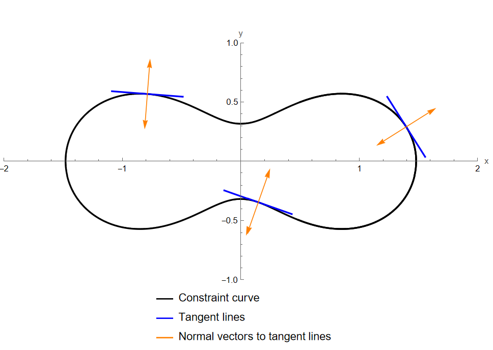
Starting at a point \(x\in I_{h}\) and moving a small distance while staying in \(I_{h}\) entails moving in a direction which lies in the tangent plane (to be more precise, for a sufficiently regular path \(x(t)\) starting at \(x(0)=x\) and staying in \(I_{h},\) the “initial direction” \(x'(0)\in\mathbb{R}^{d}\) must lie in the tangent plane at \(x\)).
The gradient \(\nabla h(x)\) is a normal vector to the tangent plane at \(x,\) i.e. a vector that is perpendicular to the tangent plane. That is, the tangent plane consists of all \(y\in\mathbb{R}^{d}\) such that \((y-x)\cdot\nabla h(x)=0.\) Figure Figure 3.1 illustrates this for \(d=2\) and constraint function \(h:\mathbb{R}^{2}\to\mathbb{R}\) given by \[h(x_{1},x_{2})=\frac{1}{(x_{1}+1)^{2}+x_{2}^{2}+1}+\frac{1}{(x_{1}-1)^{2}+x_{2}^{2}+1}-\frac{9}{10}.\] Since \(d=2,\) the constraint \(h(x_{1},x_{2})=0\) defines a curve in the plane, and the tangent planes are lines.
Heuristic derivation of condition which constrained local minima must satisfy
Let us superimpose Figure Figure 3.2, showing the curve defined by the constraint \(h(x)=0,\) onto Figure Figure 3.1, showing the (fastest descent) directions of the objective function \(f(x).\) The result is the following figure.
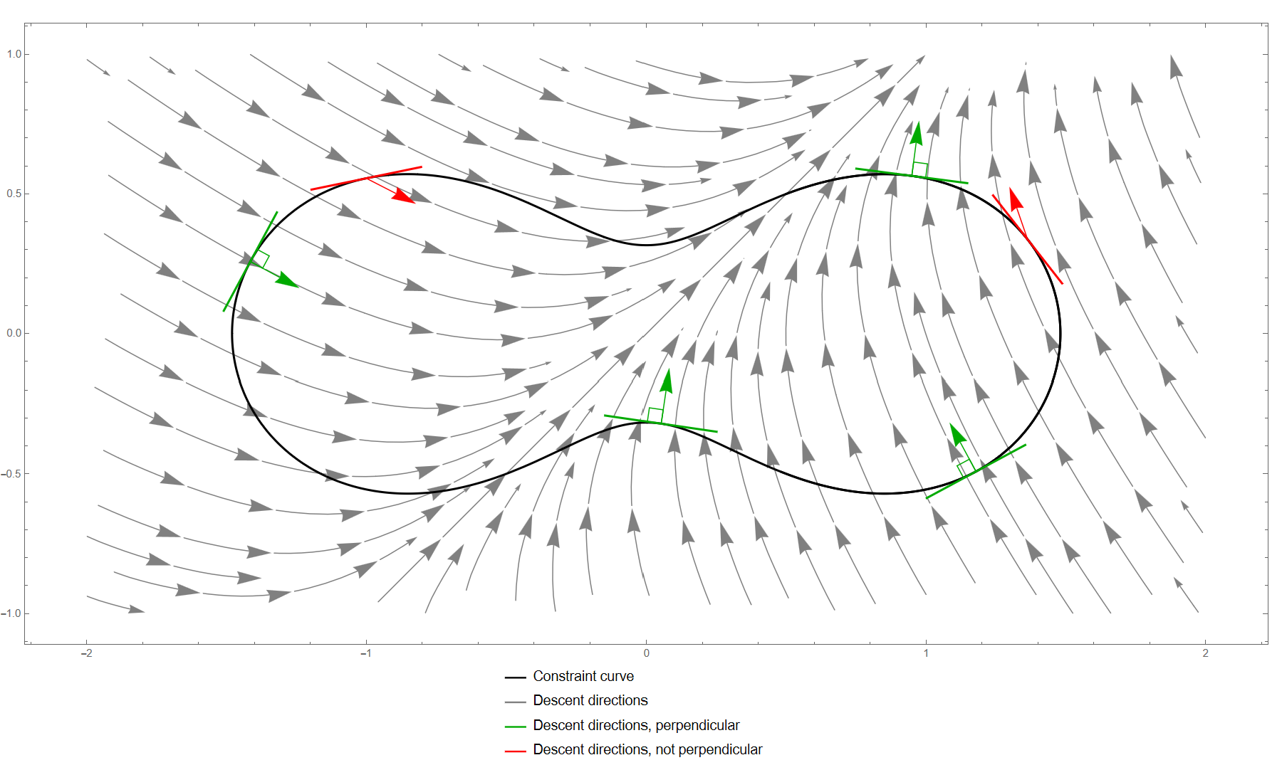
Fixing a starting point \(x\in I_{h}\) on the constraint surface and moving a small distance irrespective of the constraint, the fastest descent is achieved if moving in the direction \(-\nabla f(x),\) and a decrease by a non-zero amount is guaranteed if moving in an direction \(v\) with a negative inner product with \(\nabla f(x).\) This argument makes sense for \(d=2\) as in Figure Figure 3.3, or for general \(d\ge2.\) If we are to move a small distance while maintaining the constraint (i.e. staying in \(I_{h}\)), the directions we can move are those in the tangent plane at \(x.\) Thus if the tangent plane at \(x\in I_{h}\) contains some direction that has a non-zero inner product with \(\nabla f(x),\) then one can move a small amount while staying in \(I_{h}\) such that \(f\) decreases strictly. Thus such an \(x\in I_{h}\) can not be a local minimum of \(f|_{I_{h}}.\) Conversely, if \(x\in I_{h}\) is a local minimum of \(f|_{I_{h}},\) then the tangent plane can not contain a vector with a non-zero inner product with \(\nabla f(x).\) But this condition is equivalent to \(\nabla f(x)\) being a normal vector to the tangent plane. Since \(\nabla h(x)\) is also a normal vector to the tangent plane, and normal vectors are unique up to multiplicative factor, this means that \(\nabla f(x)\) and \(\nabla h(x)\) must be collinear. That is there should exist a \(\lambda\in\mathbb{R}\) (the Lagrange multiplier) such that \[\nabla f(x)=\lambda\nabla h(x).\tag{3.7}\] Thus, under “normal circumstances”, a local minimum of \(f|_{I_{h}}\) should satisfy the equation ([eq:ch1_loc_min_cond_for_one_eq_constraint]). Note that if you can strictly decrease \(f\) by moving in one direction on the constraint surface, then you can strictly increase it by moving in the opposite direction along the surface. Thus local maxima should also satisfy the condition ([eq:ch1_loc_min_cond_for_one_eq_constraint]).
Using method of Lagrange multipliers
Now that we understand why local extrema of \(f\) subject to the constraint \(h(x)=0\) should satisfy ([eq:ch1_loc_min_cond_for_one_eq_constraint]), let us discuss how to use that equation in practice. To find potential local minima and maxima we solve for \(x\) and \(\lambda\) in the system of equations \[\begin{cases} \nabla f(x)=\lambda\nabla h(x),\\ h(x)=0. \end{cases}\tag{3.8}\] In Figure Figure 3.3, the solutions of ([eq:ch1_intuitively_derived_first_order_condition]) are precisely the green dots on the constraint curve. The following figure plots the value of \(f(x)\) along the curve \(h(x)=0\) for the example in Figures Figure 3.1-Figure 3.3. One can observe that the green dots indeed correspond precisely to the local minima and local maxima.
The equation \(\nabla f(x)=\lambda\nabla h(x)\) by itself is an unconstrained equation, which makes it easier to solve. Often one first solves for \(x\) in this equation for fixed \(\lambda,\) obtaining a family of solutions \(x(\lambda)\) indexed by \(\lambda.\) One then plugs a solution \(x(\lambda)\) into the second line of ([eq:ch1_intuitively_derived_first_order_condition]), and obtains an equation \(h(x(\lambda))=0\) for \(\lambda.\) The latter is also an unconstrained equation! If we find a solution \(\lambda_{*}\) of it, then \(x_{*}=x(\lambda_{*})\) satisfies the constraint and also the equation \(\nabla f(x_{*})=\lambda_{*}\nabla g(x_{*}),\) and is thus a candidate for the global optimizer of the constrained optimization problem.
Thus we have reduced the problem finding constrained local extrema to solving the two unconstrained equations ([eq:ch1_intuitively_derived_first_order_condition]) in sequence. This technique is the constrained analogue of solving the critical point equation \(\nabla f(x)=0\) in unconstrained optimization.
Consider the optimization problem \[\text{minimize }\:\:x+2y\:\:\text{ subject to }\:\:x^{2}+\frac{1}{2}y^{2}=1.\tag{3.9}\] It has objective function \(f(x,y)=x+2y\) and constraint function \(h(x,y)=x^{2}+\frac{1}{2}y^{2}-1.\) We seek local minima on the curve \(h(x,y)=0\) by solving \[\nabla f(x,y)=\lambda\nabla h(x,y)\quad\text{for}\quad\text{arbitrary fixed }\lambda\in\mathbb{R}.\tag{3.10}\] We have \[\nabla f(x,y)=\left(\begin{matrix}1\\ 2 \end{matrix}\right)\quad\text{and}\quad\nabla h(x,y)=\left(\begin{matrix}2x\\ y \end{matrix}\right).\] Thus the equation ([eq:ch1_constrained_eq_first_ex_crit_point]) for this optimization problem is the system of scalar equations \[\begin{cases} 1=\lambda2x,\\ 2=\lambda y, \end{cases}\tag{3.11}\] with unique solution \[(x(\lambda),y(\lambda))=\left(\frac{1}{2\lambda},\frac{2}{\lambda}\right),\tag{3.12}\] (when \(\lambda\ne0,\) and without solution when \(\lambda=0\)). We now solve \[h(x(\lambda),y(\lambda))=0\] in \(\lambda,\) to find the potential local minima on the constraint curve. Concretely, this equation reads \[x(\lambda)^{2}+\frac{1}{2}y(\lambda)^{2}=1\quad\quad\text{i.e.}\quad\quad\frac{1}{(2\lambda)^{2}}+\frac{1}{2}\left(\frac{2}{\lambda}\right)^{2}=1.\] This equation is easy to solve by multiplying both sides by \(\lambda^{2},\) and the full set of solutions is \(\lambda=\pm\frac{3}{2}.\) Thus \[(x,y)=\pm\left(\frac{1}{3},\frac{4}{3}\right)\tag{3.13}\] are potential local minima of the objective function restricted to the curve \(h(x,y)=0.\) Plugging ([eq:ch1_constrained_eq_first_computaional_examp_x_y_sol]) into \(f\) we see that the value of the objective function at these points is \[f\left(\pm\frac{1}{3},\pm\frac{4}{3}\right)=\pm\frac{1}{3}+2\left(\pm\frac{4}{3}\right)=\pm3.\] Thus we expect \(-3\) to be the value of the optimization problem ([eq:ch1_constrained_eq_first_computaional_examp]), with minimizer given by \((x,y)=\) \(-\left(\frac{1}{3},\frac{4}{3}\right).\) Similarly, we expect the global maximum of \(f(x)\) on the curve \(h(x)=0\) to be \(3,\) with maximizer at \((x,y)=\left(\frac{1}{3},\frac{4}{3}\right).\) The figure below confirms the correctness of these conclusions.
Note that the above computation does not yet constitute a rigorous proof of these conclusions about the constrained global minimum and maximum. Indeed, below we will see that the procedure used here can fail to correctly identify the global minimum/maximum. We will also study conditions under which the procedure is guaranteed to be successful, which will turn the above computation into a rigorous proof.
3.2 Lagrange multipliers with multiple equality constraints
The problem \[\text{maximize }\,\:(x-y)^{2}-x-y+z\,\:\text{ subject to }\,\:\begin{cases} \left(x-\frac{1}{4}\right)^{2}+2y^{2}+z^{2}=1,\\ x+y+z=1, \end{cases}\tag{3.15}\] is a optimization problem with two equality constraints. The general problem with objective function \(f:\mathbb{R}^{d}\to\mathbb{R}\) and \(k\) constraint functions \(h_{i}:\mathbb{R}^{d}\to\mathbb{R}\) takes the form \[\text{minimize }\:f(x)\:\text{ subject to }\,h_{i}(x)=0\text{ for all }i=1,\ldots,k.\tag{3.16}\] A more compact formulation is to let \(h:\mathbb{R}^{d}\to\mathbb{R}^{k}\) be the function \((h_{1},\ldots,h_{k}),\) so that all \(k\) scalar constraints ([eq:ch3_multiple_equality_constraints]) are combined in the vector constraint \(h(x)=0.\) Then ([eq:ch3_multiple_equality_constraints]) is written as \[\text{minimize }\:f(x)\:\text{ subject to }h(x)=0.\tag{3.17}\] The Lagrange multiplier method generalizes to these problems, whereby the equation that local extrema satisfy is \[\nabla f(x)=\sum_{i=1}^{k}\lambda_{i}\nabla h_{i}(x)\tag{3.18}\] for the \(k\) Laplace multipliers \(\lambda_{1},\ldots,\lambda_{k}.\) To see why this condition makes sense, note that a surface \(I_{h}\) defined by \(h_{1}(x)=\ldots=h_{k}(x)=0\) will usually be \(d-k\) dimensional, with tangent space of dimension \(k.\) This tangent space is perpendicular to the \(d-k\) dimensional normal space. Under appropriate conditions, the normal space at a point \(x\) is the subspace of \(\mathbb{R}^{d}\) spanned by \(\nabla h_{1}(x),\ldots,\nabla h_{k}(x).\) Thus ([eq:ch3_multiple_equality_constraints_lagrange_equation]) is an expression of the fact that for a local extremum \(x\) of \(f|_{I_{h}}\) the fastest descent direction \(-\nabla f\) should be perpendicular to the tangent space, i.e. it should lie in the normal space. This naturally generalizes equation ([eq:ch1_loc_min_cond_for_one_eq_constraint]) from the case of \(k=1\)-dimensional normal space and \(d-1\) dimensional tangent space to the case of \(k\)-dimensional normal space and \(d-k\) dimensional tangent space.
Consider the optimization problem \[\text{maximize }\:\:c\:\:\text{ subject to }\,\,\begin{cases} \frac{1}{2}(a^{2}+b^{2}+c^{2})=1,\text{ and}\\ a+b+c=\frac{1}{2}. \end{cases}\tag{3.19}\] The objective function is \(f(a,b,c)=c\) with \[\nabla f(a,b,c)=\left(\begin{matrix}0\\ 0\\ 1 \end{matrix}\right)\] and the constraint functions are \(h_{1}(a,b,c)=\frac{1}{2}(a^{2}+b^{2}+c^{2})-1\) and \(h_{2}(a,b,c)=a+b+c-\frac{1}{2}\) with \[\nabla h_{1}(a,b,c)=\left(\begin{matrix}a\\ b\\ c \end{matrix}\right)\quad\text{and}\quad\nabla h_{2}(a,b,c)=\left(\begin{matrix}1\\ 1\\ 1 \end{matrix}\right).\] In this problem the Lagrange multiplier equation ([eq:ch3_multiple_equality_constraints_lagrange_equation]) is thus the system \[\left(\begin{matrix}0\\ 0\\ 1 \end{matrix}\right)=\lambda_{1}\left(\begin{matrix}a\\ b\\ c \end{matrix}\right)+\lambda_{2}\left(\begin{matrix}1\\ 1\\ 1 \end{matrix}\right)\] of three scalar equations. For \(\lambda_{1}=\lambda_{2}=0\) there are no solutions \((a,b,c)\) to these equations. Likewise, for \(\lambda_{1}=0,\lambda_{2}\ne0\) there are no solutions. If \(\lambda_{1}\ne0\) the unique solution is \[x(\lambda_{1},\lambda_{2}):=\left(\begin{matrix}a(\lambda_{1},\lambda_{2})\\ b(\lambda_{1},\lambda_{2})\\ c(\lambda_{1},\lambda_{2}) \end{matrix}\right):=\left(\begin{matrix}-\frac{\lambda_{2}}{\lambda_{1}}\\ -\frac{\lambda_{2}}{\lambda_{1}}\\ \frac{1-\lambda_{2}}{\lambda_{1}} \end{matrix}\right).\] For any \(\lambda_{1}\ne0,\lambda_{2}\in\mathbb{R},\) it holds that \(\nabla f(x(\lambda_{1},\lambda_{2}))=\lambda_{1}\nabla h_{1}(x(\lambda_{1},\lambda_{2}))+\lambda_{2}\nabla h_{2}(x(\lambda_{1},\lambda_{2})).\) Next we solve the equations \(h_{1}(x(\lambda_{1},\lambda_{2}))=h_{2}(x(\lambda_{1},\lambda_{2}))=0\) in \(\lambda_{1},\lambda_{2}.\) Using the form \(h_{1},h_{2}\) and \(x(\lambda_{1},\lambda_{2})\) we see that these equations reduce to \[\begin{cases} \frac{\lambda_{2}^{2}}{\lambda_{1}^{2}}+\frac{1}{2}\frac{(1-\lambda_{2})^{2}}{\lambda_{1}^{2}}=1,\\ -2\frac{\lambda_{2}}{\lambda_{1}}+\frac{1-\lambda_{2}}{\lambda_{1}}=\frac{1}{\sqrt{2}}. \end{cases}\] The second equation implies \(\sqrt{2}(1-3\lambda_{2})=\lambda_{1},\) which with the fist equation gives \[\lambda_{2}^{2}+\frac{1}{2}(1-\lambda_{2})^{2}=2(1-3\lambda_{2})^{2}.\] This equation has solutions \[\lambda_{2}=\frac{1\pm\sqrt{\frac{2}{11}}}{3}.\] Plugging these into \(\sqrt{2}(1-3\lambda_{2})=\lambda_{1}\) and solving for \(\lambda_{1}\) yields \[\lambda_{1}=\mp\frac{2}{\sqrt{11}}.\] We thus have found the (candidates for) local extrema \[(a,b,c)=\left(\frac{\sqrt{11}+\sqrt{2}}{6},\frac{\sqrt{11}+\sqrt{2}}{6},-\frac{\sqrt{11}}{3}+\frac{\sqrt{2}}{6}\right)\] and \[(a,b,c)=\left(-\frac{\sqrt{11}-\sqrt{2}}{6},-\frac{\sqrt{11}-\sqrt{2}}{6},\frac{\sqrt{11}}{3}+\frac{\sqrt{2}}{6}\right).\] Plugging these into \(f(a,b,c)\) we obtain the corresponding values of the objective function as \[-\frac{\sqrt{11}}{3}+\frac{\sqrt{2}}{6}\quad\text{and}\quad\frac{\sqrt{11}}{3}+\frac{\sqrt{2}}{6}.\] Since the latter is larger we expect it to be the value of ([eq:ch1_constrained_eq_first_computaional_examp-1]) (the former should be the result of minimizing \(c\) subject to the same constraints).
As for Example 3.1, this computation does not yet constitute a rigorous proof that the result is indeed the global minimum of the optimization problem.
3.3 Lagrange multiplier theorem
We will now formulate a rigorous theorem that provides conditions on \(f\) and \(h\) which guarantee that all local extrema \(x\) of \(f|_{I_{h}}\) are solutions of the Lagrange equation ([eq:ch3_multiple_equality_constraints_lagrange_equation]), for some values of the Lagrange multipliers \(\lambda_{1},\ldots,\lambda_{k}.\) Beyond differentiability of \(f,h,\) the condition we need is that the gradients \(\nabla h_{1}(x),\ldots,\nabla h_{k}(x)\) of each of the \(k\) constraint functions are linearly independent for all \(x\in I_{h}.\)
Let \(d\ge k\ge1\) and \(D\subset\mathbb{R}^{d}\) be open, and let \(f:D\to\mathbb{R}\) and \(h_{i}:D\to\mathbb{R},i=1,\ldots,k,\) be continuously differentiable. Let \(I_{h}=\{x\in D:h_{1}(x)=\ldots=h_{k}(x)=0\}.\) If \(x\in I_{h}\) is a local extremum of \(f|_{I_{h}}\) and \(\nabla h_{1}(x),\ldots,\nabla h_{k}(x)\in\mathbb{R}^{d}\) are linearly independent, then there exists a vector \(\lambda\in\mathbb{R}^{d}\) such that \[\nabla f(x)=\sum_{i=1}^{d}\lambda_{i}\nabla h_{i}(x).\tag{3.21}\]
If the condition of theorem is satisfied, the method of Lagrange multipliers is guaranteed to find all constrained local extrema (and thus also the constrained global extrema).
When \(k=1\) the condition that “\(\nabla h_{1}(x)\) is linearly independent” is just an unusual way to express the condition \({\nabla h_{1}(x)\ne0}.\)
Proof. Assume \(x_{*}\) is a local extremum of \(f|_{I_{h}}\) - in particular assume that \(h(x_{*})=0.\) By the condition of the theorem \(\nabla h_{1}(x_{*}),\ldots,\nabla h_{k}(x_{*})\in\mathbb{R}^{d}\) are linearly independent. Thus there exists a subset \(K\) of the coordinate indices \(\{1,\ldots,d\}\) of size \(k\) such that the \(k\times k\) matrix \((\partial_{j}h_{i}(x_{*}))_{i=1,\ldots,k,j\in K}\) has full rank. Write \(e_{1},\ldots,e_{d}\) for the standard basis vectors of \(\mathbb{R}^{d}.\) Let us change (permute) the basis so that the basis vectors \(e_{j},j\in K\) are mapped to \(e_{1},\ldots,e_{k}.\) In this new basis, it is the \(k\times k\) matrix \(A:=(\partial_{j}h_{i}(x_{*}))_{i,j=1,\ldots,k}\) that has full rank. In the rest of the proof all vectors and matrices are written in the new basis
We now use the implicit function theorem to parameterize the constraint set in a neighborhood of \(x_{*}.\) Let \(m=d-k\) and consider the map \[H:\mathbb{R}^{k}\times\mathbb{R}^{m}\to\mathbb{R}^{k}\] given by \[H(u,v)=h(\underset{\in\mathbb{R}^{d}}{\underbrace{(u,v)}}),\quad\text{for }u\in\mathbb{R}^{k},v\in\mathbb{R}^{m}.\] Then \(H\) is continuously differentiable since \(h\) is. Denote by \(D_{u}H=(\partial_{j}h_{i}((u,v)))_{i,j=1,\ldots,k}\) the Jacobian of \(H\) w.r.t. to \(u,\) which is a \(k\times k\) matrix whose \(i\)-th row consists of the first \(k\) coordinates of \(\nabla h_{i}((u,v)).\) Denote by \(D_{v}H=(\partial_{\acute{\imath}}h_{j}((u,v)))_{i=k+1,\ldots d,j=1,\ldots,k}\) the Jacobian w.r.t. to \(v,\) which is a \(k\times m\) matrix whose \(i\)-th row consists of the last \(m\) coordinates of \(\nabla h_{i}((u,v)).\)
For fixed \(v\in\mathbb{R}^{m}\) consider the equation \[H(u,v)=0\quad\text{for the unknown}\quad u\in\mathbb{R}^{k}.\tag{3.22}\] Writing any point \(x\) on the constraint surface as \(x=(u',v')\) for \(u'\in\mathbb{R}^{k},v'\in\mathbb{R}^{m},\) the point \(u=u'\) is a solution to the equation ([eq:ch3_langrange_mult_thm_implicit_eq]). In particular, letting \(u_{*}\in\mathbb{R}^{k},v_{*}\in\mathbb{R}^{m}\) be s.t. \(x_{*}=(u_{*},v_{*})\) we have \[H(u_{*},v_{*})=0.\] Now consider solutions \(\overline{u}(v)\) to([eq:ch3_langrange_mult_thm_implicit_eq]) for \(v\) close to \(v_{*}.\) Letting \(J_{u}:=D_{u}H|_{(u,v)=(u_{*},v_{*})}\) and \(J_{v}=D_{v}H|_{(u,v)=(u_{*},v_{*})}\) denote the Jacobians w.r.t. to \(u\) and \(v\) at \((u_{*},v_{*}),\) Taylor expansion yields the approximation \[H(u,v)\approx\underset{=0\in\mathbb{R}^{k}}{\underbrace{H(u_{*},v_{*})}}+\underset{k\times m}{\underbrace{J_{v}}}\underset{\in\mathbb{R}^{m}}{\underbrace{(v-v_{*})}}+\underset{k\times k}{\underbrace{J_{u}}}\underset{\in\mathbb{R}^{k}}{\underbrace{(u-u_{*})}}\] for \(u,v\) close to \(u_{*},v_{*}.\) This suggests that \((u,v)\) close to \((u_{*},v_{*})\) s.t. that \(H(u,v)=0,\) are approximated by solutions to the linear equation \(J_{v}(v-v_{*})+J_{u}(u-u_{*})=0.\) Now \(J_{u}=A\) is non-degenerate, so the latter equation has the unique solution \(u-u_{*}=-J_{u}^{-1}J_{v}(v-v_{*}),\) indicating that solutions \(\overline{u}(v)\) of ([eq:ch3_langrange_mult_thm_implicit_eq]) exist for \(v\) close to \(v_{*},\) and that \(\overline{u}(v)\approx u_{*}+J_{u}^{-1}J_{v}(v-v_{*}).\) The rigorous version of this heuristic approximation uses the implicit function theorem. Since \(H\) is continuously differentiable and \(J_{u}\) is non-degenerate, the implicit function theorem implies the existence of open balls \(U,V\) s.t \(u_{*}\in U\subset\mathbb{R}^{k},v_{*}\in V\subset\mathbb{R}^{m}\) and a continuously differentiable function \(\overline{u}:V\to U\) such that \[u\in U,v\in V,H(u,v)=0\iff u\in U,v\in V,u=\overline{u}(v).\] In particular, \[u_{*}=\overline{u}(v_{*})\quad\text{and}\quad x_{*}=(\overline{u}(v_{*}),v_{*}).\] Furthermore the Jacobian \(D\overline{u}=(\partial_{j}\overline{u}_{i}(v))_{i=1,\ldots,k,j=1,\ldots,m}\in\mathbb{R}^{k\times m}\) of \(\overline{u}\) evaluated at \(v=v_{*}\) satisfies \[\underset{k\times m}{\underbrace{D\overline{u}|_{v=v_{*}}}}=-\underset{k\times k}{\underbrace{J_{u}^{-1}}}\underset{k\times m}{\underbrace{J_{v}}}.\tag{3.23}\] (the natural formula from the point of view of the aforementioned heuristic approximation \(\overline{u}(v)\approx u_{*}+J_{u}^{-1}J_{v}(v-v_{*})\)).
Consider the continuously differentiable map \(\overline{f}:V\to\mathbb{R}\) given by \[\overline{f}(v)=f(\overline{u}(v),v).\] If \(x_{*}\) is a local minimum of \(f|_{I_{h}},\) then \(v_{*}\) must be a local minimum of \(\overline{f}.\) Similarly, if \(x_{*}\) is a local maximum then \(v_{*}\) is a local maximum of \(f.\) In either case, Lemma 2.6 implies that \[\{\nabla_{v}\overline{f}\}(v_{*})=0.\tag{3.24}\] Write \(\partial_{u_{i}}f\) for \(\partial_{i}f\) for \(i=1,\ldots,k\) and \(\nabla_{u}f=(\partial_{u_{1}}f,\ldots,\partial_{u_{k}}f)\in\mathbb{R}^{k},\) and similarly \(\partial_{v_{i}}f\) for \(\partial_{k+i}f\) for \(i=1,\ldots,m\) and \(\nabla_{v}f=(\partial_{v_{1}}f,\ldots,\partial_{v_{m}}f)\in\mathbb{R}^{m}.\) Then \(\nabla f=(\nabla_{u}f,\nabla_{v}f).\) By the chain rule \[\partial_{i}\overline{f}(v)=\sum_{j=1}^{k}\{\partial_{i}\overline{u}_{j}\}(v)\{\partial_{u_{j}}f\}(\overline{u}(v),v)+\{\partial_{v_{i}}f\}(\overline{u}(v),v),\] for \(i=1,\ldots,m,\) or in vector notation \[\underset{\in\mathbb{R}^{m}}{\underbrace{\nabla_{v}\overline{f}(v)}}=\underset{m\times k}{\underbrace{(D\overline{u}|_{v})^{T}}}\underset{\in\mathbb{R}^{k}}{\underbrace{\{\nabla_{u}f\}(\overline{u}(v),v)}}+\underset{\in\mathbb{R}^{m}}{\underbrace{\{\nabla_{v}\}f(\overline{u}(v),v)}}.\] Thus ([eq:ch3_lagrange_thm_parametrization_crit_point]) implies that \[\underset{m\times k}{\underbrace{(D\overline{u}|_{v=v_{*}})^{T}}}\underset{\in\mathbb{R}^{k}}{\underbrace{\{\nabla_{u}f\}(x_{*})}}=-\underset{\in\mathbb{R}^{m}}{\underbrace{\{\nabla_{v}f\}(x_{*})}},\] which by ([eq:langrange_thm_u_deriv]) in turn implies \[\underset{m\times k}{\underbrace{J_{v}^{T}}}\underset{k\times k}{\underbrace{(J_{u}^{-1})^{T}}}\underset{\in\mathbb{R}^{k}}{\underbrace{\{\nabla_{u}f\}(x_{*})}}=\underset{\in\mathbb{R}^{m}}{\underbrace{\{\nabla_{v}f\}(x_{*})}}.\] Letting \(\lambda=(J_{u}^{-1})^{T}\{\nabla_{u}f\}(x_{*})\in\mathbb{R}^{k}\) and using that the columns of \(J_{v}^{T}\) are the vectors \(\nabla_{v}h_{i}(x_{*}),i=1,\ldots,k\) it follows that \[\nabla_{v}f(x_{*})=\sum_{i=1}^{k}\nabla_{v}h_{i}(x_{*})\lambda_{i}.\tag{3.25}\] Furthermore \(\{\nabla_{u}f\}(x_{*})=J_{u}^{T}\lambda,\) which similarly implies that \[\nabla_{u}f(x_{*})=\sum_{i=1}^{k}\nabla_{u}h_{i}(x_{*})\lambda_{i}.\tag{3.26}\] Combining ([eq:lagrange_thm_v_part]) and ([eq:lagrange_thm_u_part]) shows that ([eq:lagrange_thm]) with \(x=x_{*}.\) Since this holds for any local minimum of \(f|_{I_{h}}\) the proof is complete.
In the proof we essentially proved that \(I_{h}\) is \(m\)-dimensional manifold, as studied in the course on differential geometry. In the language of differential geometry, the condition ([eq:lagrange_thm]) is equivalent to the covariant gradient of the function vanishes at \(x.\)
In Example 3.1, the single constraint function \(h(x,y)=x^{2}+\frac{1}{2}y^{2}-1\) has a non-zero gradient everywhere except at \(x=y=0.\) Since this point does not lie in the constraint set, the conditions of Theorem 3.1 are satisfied. Thus we can be certain that in finding all solutions of the equation [eq:ch1_constrained_eq_first_ex_crit_point] we have examined all local minimizers. Since the constraint set is compact, one of these must be a global minimizer. Thus with Theorem 3.1 the argument of Example 3.1 turns into a rigorous proof.
In Example 3.2 the two constraint functions \(h_{1}(a,b)=\frac{1}{2}(a^{2}+b^{2}+c^{2})-1\) and \(h_{2}(a,b)=a+b+c-\frac{1}{2}\) have gradients \(\nabla h_{1}(a,b)=(a,b,c)\) and \(\nabla h_{2}(a,b)=(1,1,1),\) which are linearly independent except if \(a=b=c.\) No such point satisfies both \(h_{1}(a,b,c)=0\) and \(h_{2}(a,b,c)=0,\) so the constraint set \(I_{h}\) contains no such point. Again since \(I_{h}\) set is closed, using Theorem 3.1 gives us absolute certainty that we indeed found the global minimizer in Example 3.1.
We now give an example where the condition of Theorem 3.3 is not satisfied, and where the method of Lagrange multipliers fails to find the global minimum.
Consider the optimization problem \[\text{minimize }\:y\text{ subject to }\frac{1}{3}(y-1)^{3}-\frac{1}{2}x^{2}=0,\] with objective function \(f(x,y)=y\) and single constraint function \(h(x,y)=\frac{1}{3}(y-1)^{3}-\frac{1}{2}x^{2}.\) We have \[\nabla f(x,y)=\left(\begin{matrix}0\\ 1 \end{matrix}\right)\quad\text{and}\quad\nabla h(x,y)=\left(\begin{matrix}x\\ (y-1)^{2} \end{matrix}\right).\] The Lagrange multiplier equation [eq:lagrange_thm] for this problem is thus \[\left(\begin{matrix}0\\ 1 \end{matrix}\right)=\lambda\left(\begin{matrix}x\\ (y-1)^{2} \end{matrix}\right).\] There is no solution for \(\lambda=0.\) If \(\lambda\ne0\) then the unique solutions are \[x(\lambda)=0\quad\quad y(\lambda)=1\pm\frac{1}{\sqrt{\lambda}}.\] For these the constraint \(\frac{1}{3}(y(\lambda)-1)^{3}-\frac{1}{2}x(\lambda)^{2}=0\) simplifies to \(\lambda^{-1}=0,\) so there is no \(\lambda\) such that \((x(\lambda),y(\lambda)\)) satisfies the constraint. Thus the method of Lagrange multipliers has failed to identify any local extremum for the problem.
The following plot of the constraint curve \(h(x,y)=0\) makes it evident that \((x,y)=(0,1)\) is the global minimum of \(f|_{I_{h}}.\)
Indeed, a point \((x,y)\) on the curve always has \(y\ge1,\) with equality only if \((x,y)=(0,1).\) Since \(f(x,y)=y\) this implies that \(z_{*}=(0,1)\) is the global minimum. It was not found by the method of Lagrange multipliers because \(\nabla f(z_{*})=(0,1)\ne0\) while \(\nabla h(z_{*})=0.\) Thus there is obviously no Lagrange multiplier \(\lambda\) such that \(\nabla f(z_{*})=\lambda\nabla h(z_{*}).\)
While in this example \(f\) and \(h\) are both continuously differentiable, the fact that \(\nabla h(z_{*})=0\) for the point \(z_{*}\) on the constraint curve means that the condition of Theorem 3.3 is not satisfied. Thus Theorem 3.3 does not contradict the failure of Lagrange multipliers in this case.
Alternatively, note the singular shape of the curve around \(z_{*},\) which is that of \(y=1+c|x|^{2/3}\) for appropriate \(c>0.\) Because of this shape, there are many distinct tangent lines to the curve at this point. This non-uniqueness invalidates the heuristic derivation in Section [sec:ch2_lagrange_mult]. This kind of singular shape is only possible at points on the curve s.t. \(\nabla h(x)=0.\)
3.4 Lagrangian function and dual optimization problem
Another perspective on Lagrange multipliers involves an auxiliary function called the Lagrangian function and a corresponding dual optimization problem. Consider the general minimization with equality constraints of the form \[\text{minimize}\:\:f(x)\:\text{subject to}\:\:h(x)=0,\tag{3.28}\] for an objective function \(f:D\to\mathbb{R}\) with domain \(D\subset\mathbb{R}^{d},\) and constraint function \(h:\mathbb{R}^{d}\to\mathbb{R}^{k}\) for some \(d,k\ge1.\) The result of this minimization problem can also be written \[\inf_{x\in D:h(x)=0}f(x).\tag{3.29}\] The Lagrangian function (or just Lagrangian) is the function \[L(x,\lambda)=f(x)+\lambda^{T}h(x),\tag{3.30}\] defined for any \(x\in D\) and \(\lambda\in\mathbb{R}^{k}.\) If \(f\)and \(h\) are differentiable, then so is \(L\) and \[\nabla_{x}\{L(x,\lambda)\}=\nabla f(x)+\lambda^{T}\nabla h(x),\quad\text{and}\quad\nabla_{\lambda}\{L(x,\lambda)\}=h(x).\tag{3.31}\] For a critical point \((x_{*},\lambda_{*})\) of \(L\) both gradients in ([eq:ch3_lagrangian_eq_constraint_crit_point_eq]) vanish, so then \(x_{*}\) satisfies the constraint \(h(x_{*})=0,\) and \(x_{*},\lambda_{*}\) satisfy the Lagrange equation ([eq:ch3_multiple_equality_constraints_lagrange_equation]) of the previous sections (after flipping the sign of \(\lambda\))! Conversely, under the conditions of Theorem 3.3, for any local optimizer \(x_{*}\) there exists a \(\lambda_{*}\) s.t. \((x_{*},\lambda_{*})\) is a critical point of \(L.\) However, the Lagrangian is well-defined also if \(f,h\) are not differentiable. The dual function of the Lagrangian is defined as \[q(\lambda)=\inf_{x\in D}L(x,\lambda),\quad\text{for }\lambda\in\mathbb{R}^{k}.\] Note that the \(\inf\) here is not subject to the constraint \(h(x)=0.\) The (likewise unconstrained) optimization problem \[\sup_{\lambda\in\mathbb{R}^{k}}q(\lambda)\] is called the dual optimization problem. In this context, the original ([eq:ch2_lagrange_dual_primal_problem]) is called the primal problem. The Lagrangian and dual function provide a variational lower bound for the minimum in ([eq:ch1_sec_lagrange_mult_one_q_constraint_problem_formulation_words]), as the following lemma proves.
Lemma 3.8. For any \(d\ge1,k\ge1,\) \(D\subset\mathbb{R}^{d}\) and \(f:D\to\mathbb{R},\) \(h:D\to\mathbb{R}^{k}\) it holds that \[\sup_{\lambda\in\mathbb{R}^{k}}q(\lambda)=\sup_{\lambda\in\mathbb{R}^{k}}\inf_{x\in D}L(x,\lambda)\le\inf_{x\in D:h(x)=0}f(x).\tag{3.33}\]
Proof. If \(h(x)=0\) then \(L(x,\lambda)=f(x)\) for all \(\lambda\in\mathbb{R}^{k}.\) Thus for all \(\lambda\) \[\inf_{x\in D:h(x)=0}L(x,\lambda)=\inf_{x\in D:h(x)=0}f(x).\] This implies that for all \(\lambda\) \[\inf_{x\in D}L(x,\lambda)\le\inf_{x\in D:h(x)=0}f(x).\] Maximizing both sides over \(\lambda\) proves ([eq:ch1_lagrange_var_LB_first_version]).
Note that the dual problem on the r.h.s. of ([eq:ch1_lagrange_var_LB_first_version]) is a double optimization, but each of them is unconstrained. We have thus removed the constraint, at the cost of adding an optimization over \(\lambda.\) In favorable situations the inequality in ([eq:ch1_lagrange_var_LB_first_version]) is in fact an equality, and the constrained minimum in ([eq:ch2_lagrange_dual_primal_problem]) can be computed by solving the dual problem. Several examples of this are given below.
For a maximization problem, the primal problem is of the form \[\sup_{x\in D:h(x)=0}f(x).\] Its dual function is \[q(\lambda)=\sup_{x\in D}L(x,\lambda),\] and the dual optimization problem is \[\inf_{\lambda\in\mathbb{R}^{k}}q(\lambda)=\inf_{\lambda\in\mathbb{R}^{k}}\sup_{x\in D}L(x,\lambda).\] The variational bound is now an upper bound for the optimal value of the primal problem, namely \[\sup_{x\in D:h(x)=0}f(x)\le\inf_{\lambda\in\mathbb{R}^{k}}q(\lambda)=\inf_{\lambda\in\mathbb{R}^{k}}\sup_{x\in D}L(x,\lambda).\tag{3.34}\]
We revisit Example 3.1, and this time approach it by considering the Lagrangian function and its dual. We write the optimization problem ([eq:ch1_constrained_eq_first_computaional_examp]) equivalently as \[\inf_{x,y\in\mathbb{R}:x^{2}+\frac{1}{2}y^{2}=1}\{x+2y\}.\tag{3.35}\] According to ([eq:ch1_lagrangian_def_first_version]) the Lagrangian for this problem is \[L((x,y),\lambda)=x+2y+\lambda\left(x^{2}+\frac{1}{2}y^{2}-1\right),\tag{3.36}\] and the dual function is \[q(\lambda)=\inf_{x,y\in\mathbb{R}}L((x,y),\lambda).\] By Lemma 3.8 we know that \[\sup_{\lambda\in\mathbb{R}}q(\lambda)=\sup_{\lambda\in\mathbb{R}}\inf_{x,y\in\mathbb{R}}L((x,y),\lambda)\le\inf_{x,y\in\mathbb{R}:x^{2}+\frac{1}{2}y^{2}=1}\{x+2y\}.\] For any fixed \(\lambda,\) the expression ([eq:ch1_constrained_eq_first_lagrange_dual_example]) is a quadratic in \(x,y.\) If \(\lambda<0,\) then the highest order terms in ([eq:ch1_constrained_eq_first_lagrange_dual_example]) tend to \(-\infty\) e.g. if \(x,y\to\infty,\) which means that \[\inf_{x,y\in\mathbb{R}}L((x,y),\lambda)=-\infty\:\:\text{ if }\:\:\lambda<0.\] If \(\lambda=0\) the same holds since \(x+2y\to-\infty\) if \(y=0,x\to-\infty.\) If \(\lambda>0,\) then the quadratic \((x,y)\to L((x,y),\lambda)\) is convex. Therefore we are guaranteed to find a global minimizer by solving the critical point equation \(\nabla_{z}L(z,\lambda)=0\) (where \(z=(x,y)\)). Since \(\partial_{x}L((x,y),\lambda)=1+2x\lambda\) and \(\partial_{y}L((x,y),\lambda)=2+y\lambda\) the critical point equation is the system \[\begin{cases} 1+2x\lambda=0,\\ 2+2y\lambda=0. \end{cases}\tag{3.37}\] This is the system ([eq:ch1_constrained_eq_first_computaional_examp_crit_eq_concrete]) we already solved in Example 3.1, up to the change of sign. It is easy to see that for \(\lambda=0\) there is no solution, and for \(\lambda=0\) the unique solution is \[(x(\lambda),y(\lambda))=\left(-\frac{1}{2\lambda},-\frac{2}{\lambda}\right),\tag{3.38}\] (cf. ([eq:ch1_constrained_eq_first_computaional_examp_crit_eq_sol])). Plugging this solution into \(L\) we obtain \[\begin{array}{ccl} L(x(\lambda),y(\lambda),\lambda) & = & -\frac{1}{2\lambda}+2\left(-\frac{2}{\lambda}\right)+\lambda\left(\left(-\frac{1}{2\lambda}\right)^{2}+\frac{1}{2}\left(-\frac{2}{\lambda}\right)^{2}-1\right)\\ & = & -\frac{9}{4\lambda}-\lambda. \end{array}\] Thus the dual function is given by \[q(\lambda)=\inf_{x,y\in\mathbb{R}}L((x,y),\lambda)=\begin{cases} -\infty & \text{if }\lambda\le0,\\ -\frac{9}{4\lambda}-\lambda & \text{\,if }\lambda>0. \end{cases}\] Thus the dual problem is \[\sup_{\lambda\in\mathbb{R}}q(\lambda)=\sup_{\lambda>0}\left\{ -\frac{9}{4\lambda}-\lambda\right\} .\] The function \(\lambda\to-\frac{9}{4\lambda}-\lambda\) has critical point equation \(\frac{9}{4\lambda^{2}}-1=0,\) which clearly has a unique positive solution \(\lambda_{*}=\frac{3}{2}.\) Since \(-\frac{9}{4\lambda}-\lambda\to-\infty\) for \(\lambda\downarrow0\) and \(\lambda\uparrow\infty,\) this must be the global maximizer (alternatively, one can easily check that \(\lambda\to-\frac{9}{4\lambda}-\lambda\) is concave by computing the second derivative, so a critical point is always a global maximizer). Thus \[\sup_{\lambda\in\mathbb{R}}q(\lambda)=-\frac{9}{4\lambda_{*}}-\lambda_{*}=-\frac{9}{4\cdot\frac{3}{2}}-\frac{3}{2}=-3.\tag{3.39}\] Note that this is precisely the value we argued was the global minimum in Example 3.1. In Example 3.6 we saw how Theorem 3.3 can be used conclude rigorously that this is indeed the global minimum.
In the alternative Lagrange dual approach, we obtain thanks to Lemma 3.8 the rigorous lower bound \[-3\le\inf_{x,y\in\mathbb{R}:x^{2}+\frac{1}{2}y^{2}=1}\{x+2y\}.\tag{3.40}\] In Example 3.1 we explicitly solved for \((x,y)\) on the curve \(x^{2}+\frac{1}{2}y^{2}=1,\) and successfully found the point \((x_{*},y_{*})=\left(-\frac{1}{3},-\frac{4}{3}\right)\) for which \(x_{*}+2y_{*}=-3.\) Using this knowledge we trivially obtain \[\inf_{x,y\in\mathbb{R}:x^{2}+\frac{1}{2}y^{2}=1}\{x+2y\}\le x_{*}+2y_{*}=-3.\tag{3.41}\] Since ([eq:ch1_first_lagrange_dual_example_final_LB]) and ([eq:ch1_first_lagrange_dual_example_previous_UB]) prove that \(-3\) is both an upper and a lower bound of the \(\inf,\) we have obtained a rigorous proof that \[\inf_{x,y\in\mathbb{R}:x^{2}+\frac{1}{2}y^{2}=1}\{x+2y\}=-3.\] The solution \((x_{*},y_{*})\) computed in Example 3.1 can also be obtain directly from computation here, as follows. Take the optimizer \(\lambda=\lambda_{*}=\frac{3}{2}\) for \(\lambda\) and plug it into ([eq:ch1_constrained_eq_first_ex_crit_point_eq_sol]), giving \[(x(\lambda_{*}),y(\lambda_{*}))=\left(-\frac{1}{2\lambda_{*}},-\frac{2}{\lambda_{*}}\right)\overset{\lambda_{*}=\frac{3}{2}}{=}\left(-\frac{1}{3},-\frac{4}{3}\right).\] We can verify that \(h(x(\lambda_{*}),y(\lambda_{*}))=0\) by simply explicitly computing \[x(\lambda_{*})^{2}+\frac{1}{2}y(\lambda_{*})^{2}-1=\left(-\frac{1}{3}\right)^{2}+\frac{1}{2}\left(-\frac{4}{3}\right)^{2}-1=\frac{1}{9}+\frac{8}{9}-1=0.\] Then \[\inf_{x,y\in\mathbb{R}:x^{2}+\frac{1}{2}y^{2}=1}\{x+2y\}\le x(\lambda_{*})+2y(\lambda_{*})=-\frac{1}{3}-2\frac{4}{3}=-3,\] reproducing ([eq:ch1_first_lagrange_dual_example_previous_UB]) without relying on the computation in Example 3.1.
Unlike in Example 3.1, here we did not explicitly solve for \(x_{*},y_{*}\) that satisfy the constraint, but somewhat “magically” the maximizer \(\lambda_{*}\) “selected” a point \(x(\lambda_{*}),y(\lambda_{*})\) satisfying the constraint. At the end of the section we will prove that under certain conditions this convenient outcome is guaranteed.
Consider the optimization problem \[\text{minimize }\:\:x^{4}-x^{2}+y^{2}\:\:\text{ subject to }\:\:x^{2}+xy=\frac{1}{16},\tag{3.43}\] or equivalently \[\inf_{x,y\in\mathbb{R}:x^{2}+xy=\frac{1}{16}}\left\{ x^{4}-x^{2}+y^{2}\right\} .\] The Lagrangian of the problem is \[L((x,y),\lambda)=x^{4}-x^{2}+y^{2}+\lambda\left(x^{2}+xy-\frac{1}{16}\right).\] We compute \[\sup_{\lambda\in\mathbb{R}}\inf_{x,y\in\mathbb{R}}L((x,y),\lambda).\] Consider first the dual function \[q(\lambda)=\inf_{x,y\in\mathbb{R}}L((x,y),\lambda).\] We have \[\begin{array}{ccl} {\displaystyle q(\lambda)} & = & {\displaystyle \inf_{x,y\in\mathbb{R}}}\left\{ x^{4}-x^{2}+y^{2}+\lambda(x^{2}+xy-\frac{1}{16})\right\} \\ & = & {\displaystyle \inf_{x\in\mathbb{R}}}\left\{ x^{4}-x^{2}+\lambda x^{2}+{\displaystyle \inf_{y\in\mathbb{R}}}\left(y^{2}+\lambda xy\right)\right\} -\frac{\lambda}{16} \end{array}\] The function \(y\to y^{2}+\lambda xy\) is quadratic and uniquely minimized by \[y=-\frac{\lambda x}{2}\tag{3.44}\] so \[{\displaystyle \inf_{y\in\mathbb{R}}}\left(y^{2}+\lambda xy\right)=\frac{\lambda^{2}x^{2}}{4}-\frac{\lambda^{2}x^{2}}{2}=-\frac{\lambda^{2}x^{2}}{4}.\] Thus \[\begin{array}{cl} {\displaystyle q(\lambda)} & =\inf_{x\in\mathbb{R}}\left\{ x^{4}-x^{2}+\lambda x^{2}-\frac{\lambda^{2}x^{2}}{4}\right\} -\frac{\lambda}{16}\\ & =\inf_{x\in\mathbb{R}}\left\{ x^{4}+x^{2}\left\{ -1+\lambda-\frac{\lambda^{2}}{4}\right\} \right\} -\frac{\lambda}{16}\\ & =\inf_{x\in\mathbb{R}}\left\{ x^{4}-x^{2}\left(\frac{\lambda}{2}-1\right)^{2}\right\} -\frac{\lambda}{16}. \end{array}\] Using the change of variables \(a=x^{2}\) the \(\inf\) over \(x\) turns into the quadratic minimization \[\inf_{a\ge0}\left\{ a^{2}-a\left(\frac{\lambda}{2}-1\right)^{2}\right\} \overset{a=\frac{1}{4}\left(\frac{\lambda}{2}-1\right)}{=}-\frac{1}{4}\left(\frac{\lambda}{2}-1\right)^{4}.\tag{3.45}\] Thus \[{\displaystyle q(\lambda)}=-\frac{1}{4}\left(\frac{\lambda}{2}-1\right)^{4}-\frac{\lambda}{16}.\] It remains to solve the dual problem \[\sup_{\lambda\in\mathbb{R}}{\displaystyle q(\lambda)}=\sup_{\lambda\in\mathbb{R}}\left\{ -\frac{1}{4}\left(\frac{\lambda}{2}-1\right)^{4}-\frac{\lambda}{16}\right\} .\] This function of \(\lambda\) clearly tends to \(-\infty\) as \(\lambda\to\pm-\infty,\) so its maximum must be a critical point, i.e. a solution of \[-\frac{1}{2}\left(\frac{\lambda}{2}-1\right)^{3}-\frac{1}{16}=0.\] It is easy to show that this equation has the unique solution \(\lambda=1.\) Thus \[\sup_{\lambda\in\mathbb{R}}\inf_{x,y\in\mathbb{R}}L((x,y),\lambda)=-\frac{1}{4}\left(\frac{1}{2}-1\right)^{4}-\frac{1}{16}=-\frac{5}{64}.\] Thanks to Lemma 3.8 we now have the lower bond \[-\frac{5}{64}\le\inf_{x,y\in\mathbb{R}:x^{2}+xy=\frac{1}{16}}\left\{ x^{4}-x^{2}+y^{2}\right\} .\tag{3.46}\] Let us try to match this with an upper bound. Plugging the solution \(\lambda=1\) into the minimizers of \(a,x,y\) from ([eq:ch1_lagrange_dual_second_computational_example_y_sol]) and ([eq:ch1_lagrange_dual_second_computational_example_a_sol]) above, we obtain \(a_{*}=\frac{1}{4}\left(\frac{1}{2}\right)^{2}=\frac{1}{8},\) \(x_{*}=\sqrt{a}=\frac{1}{2\sqrt{2}}\) and \(y_{*}=-\frac{1\cdot\frac{1}{2\sqrt{2}}}{2}=-\frac{1}{4\sqrt{2}}.\) We can directly verify that \[x_{*}^{2}+x_{*}y_{*}=\left(\frac{1}{2\sqrt{2}}\right)^{2}+\frac{1}{2\sqrt{2}}\left(-\frac{1}{4\sqrt{2}}\right)=\frac{1}{8}-\frac{1}{16}=\frac{1}{16},\] so \((x_{*},y_{*})\) satisfy the constraint. Thus \[\inf_{x,y\in\mathbb{R}:x^{2}+xy=\frac{1}{16}}\left\{ x^{4}-x^{2}+y^{2}\right\} \le x_{*}^{4}-x_{*}^{2}+y_{*}^{2}.\] Furthermore \[x_{*}^{4}-x_{*}^{2}+y_{*}^{2}=\frac{1}{64}-\frac{1}{8}+\frac{1}{32}=-\frac{5}{64}.\] This indeed matches the lower bound ([eq:ch1_lagrange_dual_second_computational_example_var_lb]), so we have proved that \[\inf_{x,y\in\mathbb{R}:x^{2}+xy=\frac{1}{16}}\left\{ x^{4}-x^{2}+y^{2}\right\} =-\frac{5}{64}.\]
Consider the optimization problem \[\text{maximize\textbf{ }}\:\:-x_{1}^{4}-2x_{2}^{4}-3x_{3}^{4}\:\:\text{ subject to }\:\:x_{1}^{2}+x_{2}^{2}+x_{3}^{2}=1,\tag{3.48}\] or equivalently \[\sup_{x\in\mathbb{R}^{3}:\frac{1}{2}|x|^{2}=1}\left\{ -x_{1}^{4}-2x_{2}^{4}-3x_{3}^{4}\right\} .\] The Lagrangian of the problem is \[L(x,\lambda)=-x_{1}^{4}-2x_{2}^{4}-3x_{3}^{4}+\lambda(x_{1}^{2}+x_{2}^{2}+x_{3}^{2}-1)\] with dual function \[q(\lambda)=\sup_{x\in\mathbb{R}^{3}}L(x,\lambda).\] We solve the dual problem \[\inf_{\lambda\in\mathbb{R}}q(\lambda)=\inf_{\lambda\in\mathbb{R}}\sup_{x\in\mathbb{R}^{3}}L(x,\lambda).\] For any \(\lambda\) \[q(\lambda)={\displaystyle \sup_{x\in\mathbb{R}}}\left\{ -x^{4}+\lambda x^{2}\right\} +{\displaystyle {\displaystyle \sup_{x\in\mathbb{R}}}}\left\{ -2x^{4}+\lambda x^{2}\right\} +{\displaystyle \sup_{x\in\mathbb{R}}}\left\{ -3x^{4}+\lambda x^{2}\right\} -\lambda.\] For \(k>0\) \[{\displaystyle \sup_{x\in\mathbb{R}}}\left\{ -kx^{4}+\lambda x^{2}\right\} \overset{x_{*}(\lambda)=\sqrt{\frac{\lambda}{2k}}}{=}\begin{cases} 0 & \text{\,if }\lambda\le0,\\ \frac{\lambda^{2}}{4k} & \,\text{ if }\lambda>0. \end{cases}\tag{3.49}\] Thus \[q(\lambda)=\sup_{x\in\mathbb{R}^{3}}L((x,y),\lambda)=\begin{cases} -\lambda & \text{if }\lambda\le0,\\ \frac{\lambda^{2}}{4}\left(1+\frac{1}{2}+\frac{1}{3}\right)-\lambda & \text{if }\lambda>0. \end{cases}\] We now minimize the r.h.s. is \(\lambda\) to solve the dual problem. If \(\lambda<0\) the r.h.s. is positive, for small \(\lambda>0\) it is negative, while for sufficiently large \(\lambda>0\) the r.h.s. is positive. Thus the maximizer satisfies the critical point equation \[\frac{\lambda}{2}\left(1+\frac{1}{2}+\frac{1}{3}\right)-1=0\iff\lambda=\lambda_{*}:=\frac{12}{11},\] so \[\inf_{\lambda\in\mathbb{R}}q(\lambda)=\inf_{\lambda\in\mathbb{R}}\sup_{x\in\mathbb{R}^{3}}L((x,y),\lambda)=\frac{\lambda_{*}^{2}}{4}\left(1+\frac{1}{2}+\frac{1}{3}\right)-\lambda_{*}=-\frac{6}{11}.\] By Lemma 3.8 \[\sup_{x\in\mathbb{R}^{3}:|x|^{2}=1}\left\{ -x_{1}^{4}-2x_{2}^{4}-3x_{3}^{4}\right\} \le-\frac{6}{11}.\] To match this lower bound, we try \(x_{k}^{2}=x_{k}(\lambda_{*})^{2}=\frac{\lambda_{*}}{2k}=\frac{6}{11k}\) for \(k=1,2,3.\) We verify directly that \[x_{1}(\lambda_{*})^{2}+x_{2}(\lambda_{*})^{2}+x_{2}(\lambda_{*})^{2}=\frac{6}{11}\left(1+\frac{1}{2}+\frac{1}{3}\right)=1,\] so \[\begin{array}{ccl} -\frac{6}{11} & = & -\frac{6^{2}}{11^{2}}\left(1+2\cdot\frac{1}{2^{2}}+3\cdot\frac{1}{3^{3}}\right)\\ & \le & -x_{1}(\lambda_{*})^{4}-2x_{2}(\lambda_{*})^{4}-3x_{2}(\lambda_{*})^{4}\\ & \le & \sup_{x\in\mathbb{R}^{3}:|x|^{2}=1}\left\{ -x_{1}^{4}-2x_{2}^{4}-3x_{3}^{4}\right\} \end{array}\] proving that \[\sup_{x\in\mathbb{R}^{3}:|x|^{2}=1}\left\{ -x_{1}^{4}-2x_{2}^{4}-3x_{3}^{4}\right\} =-\frac{6}{11}.\]
The next lemma explains why we could read off a constrained minimizer from the optimization of the dual in the above examples.
Lemma 3.12. Assume that \(f,g\) are continuously differentiable, and that there exists a \(\lambda_{*}\) such that \[\sup_{\lambda\in\mathbb{R}^{k}}\inf_{x\in D}L(x,\lambda)=\inf_{x\in D}L(x,\lambda_{*}).\tag{3.51}\] Assume furthermore that there is an open ball \(U\) centered at \(\lambda_{*}\) and a differentiable function \(\lambda\to x(\lambda),\) such that for all \(\lambda\in U\) the point \(x(\lambda)\) is a global minimum of \(\inf_{x\in D}L(x,\lambda)\) . Then letting \(x_{*}=h(\lambda_{*})\) it holds that \(h(x_{*})=0\) and \[\inf_{x\in D:h(x)=0}f(x)=f(x_{*})=L(x_{*,}\lambda_{*})=\sup_{\lambda\in\mathbb{R}^{k}}\inf_{x\in D}L(x,\lambda).\tag{3.52}\]
Proof. For \(\lambda\in U\) we have by assumption \[\inf_{x\in D}L(x,\lambda)=L(x(\lambda),\lambda).\] Since we have assumed \(f(x),h(x),x(\lambda)\) are all differentiable, so is \(L(x(\lambda),\lambda).\) Since \(\lambda_{*}\) is a minimizer of this function, it must hold that \[\nabla_{\lambda}\{L(x(\lambda),\lambda)\}|_{\lambda=\lambda_{*}}=0.\] By the chain rule \[\nabla_{\lambda}\{L(x(\lambda),\lambda)\}=(\{\nabla_{x}L\}(x(\lambda),\lambda))\cdot\nabla_{\lambda}\{x(\lambda)\}+\{\nabla_{\lambda}L\}(x(\lambda),\lambda).\] Since \(x(\lambda)\) is a optimizer of \(\inf_{x\in D}L(x,\lambda),\) it follows that \((\{\nabla_{x}L\}(x(\lambda),\lambda))=0\) for all \(\lambda\in U.\) Thus it must hold that \(\{\nabla_{\lambda}L\}(x_{*},\lambda_{*})=0.\) But note that \[\{\nabla_{\lambda}L\}(x,\lambda)=h(x).\] Thus we can deduce that \(h(x_{*})=0,\) proving the first claim. Furthermore \[\inf_{x\in D:h(x)=0}f(x)\le f(x_{*})=L(x_{*},\lambda_{*})\overset{(\ref{eq:lagrange_mult_dual_if_optimizer_exists_then_strong_duality_assumption})}{=}\sup_{\lambda\in\mathbb{R}^{k}}\inf_{x\in D}L(x,\lambda).\] Together with Lemma 3.8 this implies ([eq:lagrange_mult_dual_if_optimizer_exists_then_strong_duality]).
In Example 3.9, we found in ([eq:ch1_constrained_eq_first_ex_crit_point_eq_sol]) the global minimizer \((x(\lambda),y(\lambda))\) of the infimum in the dual function, and it is clearly differentiable in a neighborhood of the maximizer \(\lambda_{*}\) of the dual problem found in ([eq:langrange_dual_1_dual_miimum]). Thus Lemma 3.12 applies and proves that the minimum of the dual problem found in ([eq:langrange_dual_1_dual_miimum]) is the true constrained global minimum, even without the computations that followed ([eq:langrange_dual_1_dual_miimum]).
Lemma 3.12 can be used similarly in Example 3.10 and Example 3.11 to shorten those calculations.
Finally, we give examples of optimization problems whose dual function satisfies \[\sup_{\lambda\in\mathbb{R}^{k}}q(\lambda)=\sup_{\lambda\in\mathbb{R}^{k}}\inf_{x\in D}L(x,\lambda)<\inf_{x\in D:h(x)=0}f(x),\tag{3.53}\] so that solving the dual optimization problems does not result in the correct value of the primal optimization (such problems can of course not satisfy the conditions of Lemma 3.12). The unfortunate minimization problems for which ([eq:ch2_duality_gap]) holds are said to feature a duality gap.
Consider the minimization problem \[\text{minimize }\:x^{2}-y^{2}\text{ subject to }\:\:x+2y=3.\tag{3.54}\] The Lagrangian is \[L((x,y),\lambda)=x^{2}-y^{2}+\lambda(x+2y-3)\] and the dual function \[q(\lambda)=\inf_{x,y\in\mathbb{R}}\{x^{2}-y^{2}+\lambda(x+2y-3)\}.\] Note that \(\lim_{y\to\infty}L((0,y),\lambda)=-\infty\) for any \(\lambda,\) so \[q(\lambda)=-\infty,\quad\text{for all }\lambda\in\mathbb{R}.\] Thus also \[\sup_{\lambda\in\mathbb{R}}q(\lambda)=-\infty.\] However, the minimum of the problem is not \(-\infty,\) which is easily seen by solving for \(x\) in the constraint to get \(y=\frac{3-x}{2},\) proving that \[\inf_{x,y\in\mathbb{R}:x+2y=3}\left\{ x^{2}-y^{2}\right\} =\inf_{x\in\mathbb{R}}\left\{ x^{2}-\left(\frac{3-x}{2}\right)^{2}\right\} .\tag{3.55}\] The expression \(x^{2}-\left(\frac{3-x}{2}\right)^{2}\) is a quadratic which clearly tends to \(\infty\) for \(x\to\pm-\infty,\) so its minimum is finite. Thus the gap \[\inf_{x,y\in\mathbb{R}:x+2y=3}\left\{ x^{2}-y^{2}\right\} -\sup_{\lambda\in\mathbb{R}^{k}}q(\lambda)\] between the true minimum and the solution of the dual problem is infinite.
Minimizing the quadratic ([eq:ch3_inf_duality_gap_example_substituted]) in \(x\) one obtains the unique minimizer \(x=-1,\) corresponding to \(y=\frac{1}{2}(3-(-1))=2.\) Thus \((x_{*},y_{*})=(-1,2)\) is the actual global minimizer of ([eq:ch1_constrained_eq_first_computaional_examp-2-1-1-1-3]). For \(\lambda=2\) this point \((x_{*},y_{*})\) is a critical point of \(L((x,y),\lambda)\) (as it must, because Theorem 3.3 applies), but it is a local maximum rather than a minimum, so it is “missed” by the minimization inside the dual function.
Consider the minimization problem \[\text{minimize }\:y^{4}\:\text{ subject to }\:\:(y-1)^{2}-x^{2}=a,\tag{3.56}\] for say \(a=\frac{1}{2}.\) The lowest point on the curve \((y-1)^{2}-x^{2}=a\) is clearly \(y=1+\sqrt{a},\) giving an objective value of \((1+\sqrt{a})^{4}.\)
Let us now investigate the result of solving the Lagrange dual problem of ([eq:ch1_constrained_eq_first_computaional_examp-2-1-1-1]). The Lagrangian is \[L((x,y),\lambda)=y^{4}+\lambda((y-1)^{2}-x^{2}-a).\] Note that for \(\lambda>0\) \[q(\lambda)=\lim_{x\to\infty}L((0,x),\lambda))=\lim_{x\to\infty}(-\lambda x^{2})=-\infty,\] while for \(\lambda=0\) \[q(0)=\inf_{x,y\in\mathbb{R}}L((x,y),\lambda)=\inf_{y\in\mathbb{R}}y^{4}=0.\] This shows that \[\sup_{\lambda\in\mathbb{R}}q(\lambda)\ge0,\] so the value of the dual problem is not \(-\infty.\) For \(\lambda<0\) \[\begin{array}{ccl} q(\lambda) & = & \inf_{x,y\in\mathbb{R}}L((x,y),\lambda)\\ & = & \inf_{y\in\mathbb{R}}L((0,y),\lambda)\\ & = & \inf_{y\in\mathbb{R}}\left\{ y^{4}+\lambda((y-1)^{2}-a)\right\} . \end{array}\] This minimum is difficult to compute exactly, but it can be bounded above by setting \(y=0,\) giving \[q(\lambda)=\lambda(1-a)\overset{a<1,\lambda<0}{<}0.\] Thus \[\sup_{\lambda\in\mathbb{R}}q(\lambda)=q(0)=0,\] so \[\sup_{\lambda\in\mathbb{R}}q(\lambda)=0<(1+\sqrt{a})^{4}=\inf_{x,y\in\mathbb{R}:(y-1)^{2}-x^{2}=a}y^{4}.\]
3.5 Primal-dual optimality and KKT conditions with only equality constraints
In this section we present a generalized version of the condition in Lemma 3.12, which also guarantees that the primal and dual problems have the same optimum. We also study its relation to the simpler to check Karush-Kuhn-Tucker (KKT) conditions.
Through out this section we assume that \[d\ge1,k\ge1,\quad D\subset\mathbb{R}^{d},\quad f:D\to\mathbb{R}\quad,h:D\to\mathbb{R}^{k},\tag{3.57}\] and we are interested in the relationship between the Lagrangian \[L(x,\lambda)=f(x)+\lambda^{T}h(x),\quad\text{for }x\in D,\lambda\in\mathbb{R}^{k}\tag{3.58}\] and the constrained optimization \[\inf_{x\in D:h(x)=0}f(x).\tag{3.59}\] First we give a version of Lemma 3.12 that does not require that \(f,h\) are differentiable. It requires instead \(x_{*}\in D,\lambda_{*}\in\mathbb{R}^{k}\) such that \[L(x_{*},\lambda)\overset{\forall\lambda\in\mathbb{R}^{k}}{\le}L(x_{*},\lambda_{*})\overset{\forall x\in D}{\le}L(x,\lambda_{*}).\tag{3.60}\] We call \((x_{*},\lambda_{*})\) that satisfies this Lagrange primal-dual optima.
Lemma 3.16 (Lagrange primal-dual optimality implies optimality subject to equality constraint). Assume ([eq:ch3_KKT_cond_eq_const_running_assumption_1])-([eq:ch3_KKT_cond_eq_const_running_assumption_3]). If \(x_{*}\in D,\lambda_{*}\in\mathbb{R}^{k}\) are s.t. \((x_{*},\lambda_{*})\) is primal-dual optimal (i.e. satisfies ([eq:lagrange_primal_dual_optimal_cond])), then \[h(x_{*})=0\tag{3.61}\] and \[\inf_{x\in D:h(x)=0}f(x)=L(x_{*},\lambda_{*})=\sup_{\lambda\in\mathbb{R}^{k}}\inf_{x\in D}L(x,\lambda).\tag{3.62}\]
Proof. We first argue that such an \(x_{*}\) must satisfy the constraint \(h(x_{*})=0.\) Indeed, for \(\Delta\in\mathbb{R}^{k}\) \[L(x_{*},\lambda_{*}+\Delta)=L(x_{*},\lambda_{*})+\Delta\cdot h(x_{*}).\] Thus if \(h(x_{*})\ne0\) then one can pick an \(\Delta\) such that \(L(x_{*},\lambda_{*}+\Delta)>L(x_{*},\lambda_{*}),\) which contradicts the left inequality of ([eq:lagrange_primal_dual_optimal_cond]). Therefore it must hold that \(h(x_{*})=0,\) so we have proved ([eq:ch3_lagrange_minimax_only_eq_constraint_feasability]).
In turn, ([eq:ch3_lagrange_minimax_only_eq_constraint_feasability]) implies that \[\inf_{x\in D:h(x)=0}f(x)\le f(x_{*})=L(x_{*},0).\] By the left inequality of ([eq:lagrange_primal_dual_optimal_cond]) it follows that \[\inf_{x\in D:h(x)=0}f(x)\le L(x_{*},\lambda_{*}).\] From the right inequality of ([eq:lagrange_primal_dual_optimal_cond]) it follows that \[L(x_{*},\lambda_{*})\le\inf_{x\in D}L(x,\lambda_{*}),\] and trivially \[\inf_{x\in D}L(x,\lambda_{*})\le\sup_{\lambda\in\mathbb{R}^{k}}\inf_{x\in D}L(x,\lambda).\] Combining these we obtain \[\inf_{x\in D:h(x)=0}f(x)\le\sup_{\lambda\in\mathbb{R}^{k}}\inf_{x\in D}L(x,\lambda).\] The matching lower bound follows from Lemma 3.8, so ([eq:ch3_lagrange_minimax_only_eq_constraint_optimality]) follows.
The primal-dual optimality condition ([eq:lagrange_primal_dual_optimal_cond]) is equivalent to \[L(x_{*},\lambda_{*})=\inf_{x\in D}L(x,\lambda_{*})=\sup_{\lambda\in\mathbb{R}^{k}}L(x_{*},\lambda).\] Some authors call a primal-dual optimal pair \((x_{*},\lambda_{*})\) a saddle point of the Lagrangian. This notion of saddle point is not consistent with that of Definition [def:ch2_critical_point_saddle_point]. To avoid confusion these notes only use saddle point in the latter sense.
However, if \(f,h\) are differentiable, then any primal-dual optimal pair \((x_{*},\lambda_{*})\) is a saddle point of \(L\) in the sense of Definition [def:ch2_critical_point_saddle_point]. The critical point conditions \(\nabla_{x}L(x,\lambda)=0,\nabla_{\lambda}L(x,\lambda)=0\) are called the Karush-Kuhn-Tucker conditions, and in our current setting take the form \[\{\nabla_{x}L\}(x_{*},\lambda_{*})=0,\tag{3.63}\] \[h(x_{*})=0.\tag{3.64}\] Later we will study KKT conditions for constrained optimization problems with inequality constraints, which include additional conditions which are not simply the critical point conditions of the Lagrangian.
Lemma 3.17 (Primal-dual optimum satisfies KKT conditions). Assume ([eq:ch3_KKT_cond_eq_const_running_assumption_1])-([eq:ch3_KKT_cond_eq_const_running_assumption_3]). If \(f\) is differentiable and \(x_{*}\in D^{\circ},\lambda_{*}\in\mathbb{R}^{k}\) is primal-dual optimal (i.e. satisfies ([eq:lagrange_primal_dual_optimal_cond])), then \((x_{*},\lambda_{*})\) satisfies the KKT conditions ([eq:KKT_COND_equ_1])-([eq:KKT_COND_equ_2]).
Proof. The previous theorem already proved that ([eq:KKT_COND_equ_2]) follows from ([eq:lagrange_primal_dual_optimal_cond]). Next, the right inequality of ([eq:lagrange_primal_dual_optimal_cond]) implies that \(x_{*}\) is a minimizer of the differentiable function \(x\to L(x,\lambda_{*}).\) By Lemma 2.6 this implies ([eq:KKT_COND_equ_1]).
The significance of Lemma 3.17 in practice is analogous to that of the critical point equation \(\nabla f(x)=0\) for unconstrained optimization: one can search for a primal-dual optimum by solving the equations ([eq:KKT_COND_equ_1])-([eq:KKT_COND_equ_2]). Note however that a primal-dual optimal pair may not exist, even for differentiable \(f,h\) .
In general, solving ([eq:KKT_COND_equ_1])-([eq:KKT_COND_equ_2]) only provides candidates for a primal-dual optimum: even if one finds all solutions to ([eq:KKT_COND_equ_1])-([eq:KKT_COND_equ_2]) one must check by some other means that a pair satisfies the condition ([eq:lagrange_primal_dual_optimal_cond]). This is analogous to unconstrained optimization, where a solution \(x\) of the critical point equation \(\nabla f(x)=0\) is in general not guaranteed to be a global optimum. Recall however that if \(f\) is convex or concave then a solution to \(\nabla f(x)=0\) is guaranteed to be a global optimum. The next result is the analogue for Lagrange primal-dual optimality: if \(f\) is convex and \(h\) affine (very strong assumptions!), any pair \((x_{*},\lambda_{*})\) that satisfies the KKT conditions is guaranteed to be primal-dual optimal.
Lemma 3.18 (KKT conditions imply primal-dual optimality for \(f\) convex, \(h\) affine.). Assume ([eq:ch3_KKT_cond_eq_const_running_assumption_1])-([eq:ch3_KKT_cond_eq_const_running_assumption_3]). In addition, assume that \(D\subset\mathbb{R}^{d}\) is convex, that \(f:D\to\mathbb{R}\) is convex and differentiable, and that \(h(x)=Ax-b\) for some \(k\times d\) matrix \(A\) and vector \(b\in\mathbb{R}^{k}.\) If \(x_{*}\in D^{\circ},\lambda_{*}\in\mathbb{R}^{k}\) are s.t. the pair \((x_{*},\lambda_{*})\) satisfy the KKT conditions ([eq:KKT_COND_equ_1])-([eq:KKT_COND_equ_2]), then \((x_{*},\lambda_{*})\) is primal-dual optimal (i.e. satisfies ([eq:lagrange_primal_dual_optimal_cond])). In particular, then \[\inf_{x\in D:Ax=b}f(x)=L(x_{*},\lambda_{*})=\sup_{\lambda\in\mathbb{R}^{k}}\inf_{x\in D}L(x,\lambda).\]
Proof. Since \(f\) is convex and \(h\) is affine, it follows that \(x\to L(x,\lambda_{*})\) is convex and differentiable. Thus Lemma 2.12 combined with ([eq:KKT_COND_equ_1]) implies that \(x_{*}\) is a global minimizer of \(x\to L(x,\lambda_{*}),\) which means that indeed \[L(x_{*},\lambda_{*})\overset{\forall x\in D}{\le}L(x,\lambda_{*}).\] This is the right side of ([eq:lagrange_primal_dual_optimal_cond]). Next if ([eq:KKT_COND_equ_2]) holds, then \(L(x_{*},\lambda)\) does not depend on \(\lambda.\) Thus the left inequality of ([eq:lagrange_primal_dual_optimal_cond]) in fact holds with equality.
3.6 Inequality constraints
The Lagrange dual approach can also accommodate inequality constraints, such as in the problem \[\text{minimize }\:-x^{4}-2y^{4}\:\text{ subject to }\:\:2x^{2}+y^{2}\le1.\tag{3.65}\] A general optimization problem with \(k\) equality constraints \(h_{1}(x)=\ldots=h_{k}(x)=0\) and \(p\) inequality constraints \(g_{1}(x)\le0,\ldots,g_{p}(x)\le0\) takes the form \[\text{minimize }\:f(x)\:\text{ subject to }\:\:h(x)=0,g(x)\le0,\] where \(h:D\to\mathbb{R}^{k}\) and \(g:D\to\mathbb{R}^{p}.\) Since \(g_{i}(x)\ge0\iff-g_{i}(x)\le0\) this form also covers inequality constraints that are lower bounds (as well as maximization problems with equality and inequality constraints).
The Lagrangian of this problem is \[L(x,\lambda,\nu)=f(x)+\lambda h(x)+\nu g(x),\quad\text{for }x\in D,\lambda\in\mathbb{R}^{k},\nu\in\mathbb{R}^{p},\] where both \(\lambda\) and \(\nu\) are called Lagrange multipliers.
The dual function is \[q(\lambda,\nu)=\inf_{x\in D}L(x,\lambda,\nu),\] and the dual optimization problem is \[\sup_{\lambda\in\mathbb{R}^{k},v\in[0,\infty)^{p}}g(\lambda,\nu).\] Note that in the dual problem the Lagrange multipliers \(\nu\) corresponding to the inequality constraints are non-negative.
The variational lower bound Lemma 3.19 straight-forwardly generalizes to the setting allowing for inequality constraints.
Lemma 3.19. For any \(d\ge1,\) \(D\subset\mathbb{R}^{d}\) and \(f:D\to\mathbb{R},h:D\to\mathbb{R}^{k},\) \(g:D\to\mathbb{R}^{p}\) it holds that \[\sup_{\lambda\in\mathbb{R}^{k},\nu\in[0,\infty)^{p}}q(\lambda,\nu)=\sup_{\lambda\in\mathbb{R}^{k},\nu\in[0,\infty)^{p}}\inf_{x\in D}L(x,\lambda)\le\inf_{x\in D:h(x)=0,g(x)\le0}f(x).\tag{3.67}\]
Proof. If \(h(x)=0\) and \(g(x)\le0,\) then \(L(x,\lambda,\nu)\le f(x)\) for all \(\lambda\in\mathbb{R}^{k},\nu\in[0,\infty)^{p}.\) Thus for all such \(\lambda,\nu\) \[\inf_{x\in D}L(x,\lambda,\nu)\le\inf_{x\in D:h(x)=0,g(x)\le0}L(x,\lambda,\nu)\le\inf_{x\in D:h(x)=0,g(x)\le0}f(x).\] Maximizing both sides over \(\lambda,\nu\) gives ([eq:ch1_lagrange_var_LB_first_version-1]).
The primal-dual optimality condition generalizes to \[L(x_{*},\lambda,\nu)\overset{\forall\lambda\in\mathbb{R}^{k},\nu\in[0,\infty)^{p}}{\le}L(x_{*},\lambda_{*},\nu_{*})\overset{\forall x\in D}{\le}L(x,\lambda_{*},\nu_{*}).\tag{3.68}\] It is equivalent to \[L(x_{*},\lambda_{*},\nu_{*})=\inf_{x\in D}L(x,\lambda_{*},\nu_{*})=\sup_{\lambda\in\mathbb{R}^{k},\nu\in[0,\infty)^{p}}L(x_{*},\lambda,\nu).\] If a triple \((x_{*},\lambda_{*},\nu_{*})\) with \(x_{*}\in D,\lambda_{*}\in\mathbb{R}^{k},\nu_{*}\in[0,\infty)^{p}\) satisfies this condition we call it a Lagrange primal-dual optimum. It is easy to show that when such an optimum exists then, then the value of primal and dual problems coincide. This generalizes Lemma [lem:ch3_lagrange_minimax_only_eq_constraint].
Lemma 3.20. Assume \(x_{*}\in D,\lambda_{*}\in\mathbb{R}^{k},\nu_{*}\in[0,\infty)^{p}\) are primal-dual optimal (i.e. satisfy ([eq:lagrange_primal_dual_optimal_cond_full_with_ineq])). Then \[h(x_{*})=0,\quad g(x_{*})\le0\tag{3.70}\] and \[\inf_{x\in D:h(x)=0,g(x)\le0}f(x)=L(x_{*},\lambda_{*},\nu_{*})=\sup_{\lambda\in\mathbb{R}^{k},\nu\in[0,\infty)^{p}}\inf_{x\in D}L(x,\lambda,\nu).\tag{3.71}\]
Proof. The proof that \(h(x_{*})=0\) is identical to in Lemma [lem:ch3_lagrange_minimax_only_eq_constraint]. Assume that \(g_{i}(x_{*})>0\) for some \(i=1,\ldots,p.\) Then taking \(\nu_{i}\to\infty\) we have \(L(x_{*},\lambda_{*},\nu)\to\infty,\) which contradicts the left inequality of ([eq:lagrange_primal_dual_optimal_cond_full_with_ineq]). Thus it must hold that \(g_{i}(x_{*})\le0\) for all \(i=1,\ldots.p.\) We have proved ([eq:ch3_primal_dual_optimality_implies_optimality_thm_feasability]).
Next, from ([eq:ch3_primal_dual_optimality_implies_optimality_thm_feasability]) it follows that \[\inf_{x:h(x)=0,g(x)\le0}f(x)\le f(x_{*}).\] Trivially we have \[f(x_{*})=L(x_{*},0,0).\] By the left inequality of ([eq:lagrange_primal_dual_optimal_cond_full_with_ineq]) it follows that \[L(x_{*},0,0)\le L(x_{*},\lambda_{*},\nu_{*}).\] Combining these yields \[\inf_{x:h(x)=0,g(x)\le0}f(x)\le L(x_{*},\lambda_{*},\nu_{*}).\] By the right inequality of ([eq:lagrange_primal_dual_optimal_cond_full_with_ineq]) it follows that \[\inf_{x:h(x)=0,g(x)\le0}f(x)\le\inf_{x\in D}L(x,\lambda_{*},\nu_{*}).\] Trivially \[\inf_{x\in D}L(x,\lambda_{*},\nu_{*})\le\sup_{\lambda\in\mathbb{R}^{k},\nu\in[0,\infty)^{p}}\inf_{x\in D}L(x,\lambda,\nu).\] This combined with Lemma 3.19 proves ([eq:ch3_primal_dual_optimality_implies_optimality_thm_optimality]).
Consider the optimization problem \[\text{Minimize }\quad x+y\quad\text{subject to }\begin{cases} x^{2}+xy+y^{2}\le1,\\ x^{2}-xy+y^{2}\le1. \end{cases}\] The Lagrangian is \[L((x,y),\nu_{1},\nu_{2})=x+y+\nu_{1}(x^{2}+xy+y^{2}-1)+\nu_{2}(x^{2}-xy+y^{2}-1).\] The dual function is \[q(\nu)=\inf_{x,y\in\mathbb{R}}L((x,y),\nu_{1},\nu_{2}).\] If \(\nu_{1}=\nu_{2}=0\) then \(\inf_{x,y\in\mathbb{R}}L((x,y),0,0)=-\infty.\) The Lagrangian \(L((x,y),\nu_{1},\nu_{2})\) is quadratic in \(x,y,\) and \[x^{2}+xy+y^{2}-1=\frac{1}{2}(x^{2}+y^{2})+\frac{1}{2}(x+y)^{2}-1\to\infty\quad\text{as}\quad(x,y)\to\infty.\] The same holds for \(x^{2}-xy+y^{2}-1.\) Thus for \(\nu_{1},\nu_{2}\ge0,\nu_{1}+\nu_{2}>0\) it holds that \(L((x,y),\nu_{1},\nu_{2})\to\infty\) as \((x,y)\to\infty.\) Thus the quadratic \((x,y)\to L((x,y),\nu_{1},\nu_{2})\) must have a unique critical point, which is the global minimum. The critical point equation for \(x,y\) is \[\begin{cases} 1+\nu_{1}(2x+y)+\nu_{2}(2x-y)=0,\\ 1+\nu_{1}(x+2y)+\nu_{2}(-x+2y)=0. \end{cases}\] Rearranging this turns into \[\begin{cases} 2(\nu_{1}+\nu_{2})x+(\nu_{1}-\nu_{2})y=-1,\\ (\nu_{1}-\nu_{2})x+2(\nu_{1}+\nu_{2})y=-1, \end{cases}\] which for \(\nu_{1},\nu_{2}\ge0,\nu_{1}+\nu_{2}>0\) has unique solution \[x=y=-\frac{1}{3\nu_{1}+\nu_{2}}.\tag{3.73}\] Write \(w=-\frac{1}{3\nu_{1}+\nu_{2}}\) for convenience, so the solution is \(x=y=w.\) Plugging the solution into the Lagrangian gives \[\begin{array}{ccl} L((x,y),\nu_{1},\nu_{2}) & = & 2w+\nu_{1}(3w^{2}-1)+\nu_{2}(w^{2}-1)\\ & = & 2w+w^{2}(3\nu_{1}+\nu_{2})-\nu_{1}-\nu_{2}\\ & = & -\frac{1}{3\nu_{1}+\nu_{2}}-v_{1}-v_{2}. \end{array}\] Thus the dual function is \[q(\nu_{1},\nu_{2})=\begin{cases} -\infty & \text{ if }\nu_{1}=\nu_{2}=0\\ -\frac{1}{3\nu_{1}+\nu_{2}}-v_{1}-v_{2} & \text{\,if }\nu_{1},\nu_{2}\ge0,\nu_{1}+\nu_{2}>0 \end{cases}\] The dual problem is \[\sup_{\nu_{1},\nu_{2}\in[0,\infty)}q(\nu_{1},\nu_{2})=\sup_{\nu_{1},\nu_{2}\in[0,\infty)}\left\{ -\frac{1}{3\nu_{1}+\nu_{2}}-v_{1}-v_{2}\right\} .\] To solve this problem, we consider the critical point equation for \(\nu_{1},\nu_{2}\): \[\begin{cases} \frac{3}{(3\nu_{1}+\nu_{2})^{2}}-1=0,\\ \frac{1}{(3\nu_{1}+\nu_{2})^{2}}-1=0. \end{cases}\] These two equations clearly have no solution. Just the supremum most be appear on the boundary, that is for \(\nu_{1}=0\) or \(\nu_{2}=0\) (\(\nu_{1}=\nu_{2}=0\) is obviously not a maximizer). Thus \[\sup_{\nu_{1},\nu_{2}\in[0,\infty)}q(\nu_{1},\nu_{2})=\max\left(\sup_{\nu_{1}\ge0}\left\{ -\frac{1}{3\nu_{1}}-\nu_{1}\right\} ,\sup_{\nu_{2}\ge0}\left\{ -\frac{1}{\nu_{2}}-\nu_{2}\right\} \right).\] It is clear that \(\sup_{\nu_{1}\ge0}\left\{ -\frac{1}{3\nu_{1}}-\nu_{1}\right\} >\sup_{\nu_{2}\ge0}\left\{ -\frac{1}{\nu_{2}}-\nu_{2}\right\} ,\) and the global maximizer of \(\sup_{\nu_{1}\ge0}\left\{ -\frac{1}{3\nu_{1}}-\nu_{1}\right\}\) is \(\nu_{1,*}=\frac{1}{\sqrt{3}},\) for which \(-\frac{1}{3v_{1,*}}-\nu_{1,*}=-\frac{2}{\sqrt{3}}.\) Letting also \(\nu_{2,*}=0\) we have \[\sup_{\nu_{1},\nu_{2}\in[0,\infty)}q(\nu_{1},\nu_{2})=q(\nu_{*,1},\nu_{*,2})=-\frac{2}{\sqrt{3}}.\] By Lemma 3.19 we obtain the lower bound \[\inf_{(x,y)\in\mathbb{R}^{2}:\begin{cases} x^{2}+xy+y^{2}\le1\\ x^{2}-xy+y^{2}\le1 \end{cases}}\{x+y\}\ge-\frac{2}{\sqrt{3}}.\] Recalling ([eq:ch3_inequlaity_constraint_first_example_x_y_sol]), let \[x_{*}=y_{*}=-\frac{1}{3\nu_{1,*}+\nu_{2,*}}=-\frac{1}{\sqrt{3}}.\] Since we successfully argued that ([eq:ch3_inequlaity_constraint_first_example_x_y_sol]) was the global optimum when minimizing over \(x,y\) we have that \[L((x_{*},y_{*}),\nu_{1,*},\nu_{2,*})\overset{\forall x,y\in\mathbb{R}}{\le}L((x,y),\nu_{1,*},\nu_{2,*})\] We also successfully argued that \((\nu_{1,*},\nu_{2,*})\) is the global maximizer in \(\sup_{\nu_{1},\nu_{2}\in[0,\infty)}q(\nu_{1},\nu_{2}),\) so we have that \[L((x_{*},y_{*}),\nu_{1},\nu_{2})\overset{\forall\nu_{1},\nu_{2}\in[0,\infty)}{\le}L((x_{*},y_{*}),\nu_{1,*},\nu_{2,*}).\] Thus the primal-dual optimality conditions ([eq:lagrange_primal_dual_optimal_cond_full_with_ineq]) holds, and by Lemma [lem:ch3_primal_dual_optimality_implies_optimality] we can conclude that \[\inf_{(x,y)\in\mathbb{R}^{2}:\begin{cases} x^{2}+xy+y^{2}\le1\\ x^{2}-xy+y^{2}\le1 \end{cases}}\{x+y\}=-\frac{2}{\sqrt{3}}.\]
In the presence of inequality constraints the Karush-Kuhn-Tucker conditions generalize to: \[\{\nabla_{x}L\}(x_{*},\lambda_{*},\nu_{*})=0,\tag{3.74}\] \[h(x_{*})=0,g_{i}(x_{*})\le0,\tag{3.75}\] \[\nu_{*}\in[0,\infty)^{p},\tag{3.76}\] \[\nu_{*,i}g_{i}(x_{*})=0\quad\text{for all }\quad i=1,\ldots,p.\tag{3.77}\] The last condition can also be stated as “\(\nu_{*,i}=0\) or \(g_{i}(x_{*})=0\) for all \(i=1,\ldots,p\)”.
Lemma 3.22 (Primal-dual optima satisfy KKT conditions). If \(f,g,h\) are differentiable and \(x_{*}\in D^{\circ},\lambda_{*}\in\mathbb{R}^{k},\nu_{*}\in[0,\infty)^{p}\) is primal-dual optimal (i.e. satisfies ([eq:lagrange_primal_dual_optimal_cond_full_with_ineq])), then \((x_{*},\lambda_{*},\nu_{*})\) satisfies the KKT conditions ([eq:KKT_COND_ineq_1])-([eq:KKT_COND_ineq_4]).
Proof. The previous theorem already proved that ([eq:KKT_COND_ineq_2]) follows from ([eq:lagrange_primal_dual_optimal_cond_full_with_ineq]). Next, the right inequality of ([eq:lagrange_primal_dual_optimal_cond_full_with_ineq]) implies that \(x_{*}\) is a minimizer of the differentiable function \(x\to L(x,\lambda_{*},\nu_{*}).\) By Lemma 2.6 this implies ([eq:KKT_COND_ineq_1]). The condition ([eq:KKT_COND_ineq_3]) is already part of the assumptions of the lemma.
To prove ([eq:KKT_COND_ineq_4]), assume that \(g_{i}(x_{*})\ne0\) and \(\nu_{*,i}\ne0.\) Since we already know that ([eq:KKT_COND_ineq_2]) holds, this means that \(g_{i}(x_{*})<0,\) and by assumption \(\nu_{*,i}>0.\) But then defining \(\nu\in[0,\infty)^{p}\) by \(\nu_{j}=\nu_{*,j}-\Delta\delta_{ij}\) for a \(0<\Delta\le\nu_{*,j},\) we have \[L(x_{*},\lambda_{*},\nu)=L(x_{*},\lambda_{*},\nu_{*})-\Delta g_{i}(x_{*})>L(x_{*},\lambda_{*},\nu_{*}).\] This contradicts the left inequality of ([eq:lagrange_primal_dual_optimal_cond_full_with_ineq]). Thus it must hold that \(g_{i}(x_{*})=0\) or \(\nu_{*,i}=0.\) This proves ([eq:KKT_COND_ineq_4]).
For the optimization problem in Example 3.21 with Lagrangian \[L((x,y),\nu_{1},\nu_{2})=x+y+\nu_{1}g_{1}(x,y)+\nu_{2}g_{2}(x,y)\] for \[g_{1}(x,y)=x^{2}+xy+y^{2}-1,\] \[g_{2}(x,y)=x^{2}-xy+y^{2}-1,\] we obtained \((x_{*},y_{*},\nu_{1,*},\nu_{2,*})=(-\frac{1}{\sqrt{3}},-\frac{1}{\sqrt{3}},\frac{1}{\sqrt{3}},0).\) We verified that it was primal-dual optimal, so Lemma 3.22 implies that the KKT conditions ([eq:KKT_COND_ineq_1])-([eq:KKT_COND_ineq_4]) must hold. Let us verify this manually. We have \[\nabla_{(x,y)}L((x,y),\nu_{1},\nu_{2})=\left(\begin{matrix}1\\ 1 \end{matrix}\right)+\nu_{1}\left(\begin{matrix}2x+y\\ x+2y \end{matrix}\right)+\nu_{2}\left(\begin{matrix}2x-y\\ -x+2y \end{matrix}\right),\] so \[\nabla_{(x,y)}L((x_{*},y_{*}),\nu_{1,*},\nu_{2,*})=\left(\begin{matrix}1\\ 1 \end{matrix}\right)+\frac{1}{\sqrt{3}}\left(\begin{matrix}-\sqrt{3}\\ -\sqrt{3} \end{matrix}\right)+0\cdot\left(\begin{matrix}2x_{*}-y_{*}\\ -x_{*}+2y_{*} \end{matrix}\right)=0.\] Thus ([eq:KKT_COND_ineq_1]) indeed holds. Furthermore \[g_{1}(x_{*},y_{*})=\left(-\frac{1}{\sqrt{3}}\right)^{3}+\left(-\frac{1}{\sqrt{3}}\right)^{3}+\left(-\frac{1}{\sqrt{3}}\right)^{3}-1=0,\] and \[g_{2}(x_{*},y_{*})=\left(-\frac{1}{\sqrt{3}}\right)^{3}-\left(-\frac{1}{\sqrt{3}}\right)^{3}+\left(-\frac{1}{\sqrt{3}}\right)^{3}-1<0,\] so ([eq:KKT_COND_ineq_2]) also holds. Finally \[\nu_{1,*}g_{1}(x_{*},y_{*})=\frac{1}{\sqrt{3}}\times0=0\] and \[\nu_{2,*}g_{2}(x_{*},y_{*})=0\times g_{2}(x_{*},y_{*})=0,\] so ([eq:KKT_COND_ineq_4]) holds.
The significance of Lemma 3.22 in practice is that one can find candidates for primal-dual optima by finding triples \((x_{*},\lambda_{*},\nu_{*})\) that satisfy the KKT conditions ([eq:KKT_COND_ineq_1])-([eq:KKT_COND_ineq_4]). Once found however, one needs to verify actual primal-dual optimality condition ([eq:lagrange_primal_dual_optimal_cond_full_with_ineq]) to be sure that one has found the true optimum of the constrained optimization. This is because the implication of Lemma 3.22 only goes one way; satisfying ([eq:KKT_COND_ineq_1])-([eq:KKT_COND_ineq_4]) does not imply that ([eq:lagrange_primal_dual_optimal_cond_full_with_ineq]) is satisfied.