0.2.7 Primal-dual optimality and Lagrange conditions
In this section we present a generalized version of the condition in Lemma 2.44, which does not require that \(f,h\) are differentiable, and which also guarantees that the primal and dual problems have the same optimum.
Through out this section we assume that \[d\ge1,k\ge1,\quad D\subset\mathbb{R}^{d},\quad f:D\to\mathbb{R}\quad,h:D\to\mathbb{R}^{k},\tag{2.51}\] and we are interested in the relationship between the Lagrangian \[L(x,\lambda)=f(x)+\lambda^{T}h(x),\quad\text{for }x\in D,\lambda\in\mathbb{R}^{k}\tag{2.52}\] and the constrained optimization \[\inf_{x\in D:h(x)=0}f(x).\tag{2.53}\] The generalized condition is the following.
\(\:\)
Consider the constrained optimization problem of (2.18), and let \(L(x,\lambda)\) be its Lagrangian. The conditions \[L(x_{*},\lambda)\overset{\forall\lambda\in\mathbb{R}^{k}}{\le}L(x_{*},\lambda_{*})\overset{\forall x\in D}{\le}L(x,\lambda_{*}),\tag{2.54}\] or equivalently \[\sup_{\lambda\in\mathbb{R}^{k}}L(x_{*},\lambda)=L(x_{*},\lambda_{*})=\inf_{x\in D}L(x,\lambda_{*}),\] for \(x\in D,\lambda\in\mathbb{R}^{k}\) are called the Lagrange primal-dual optimality conditions Any \((x_{*},\lambda_{*})\in D\times\mathbb{R}^{k}\) that satisfies the condition is called a Lagrange primal-dual optimum.
\(\,\)
Let \(f,D,g\) be as in the constrained minimization problem (2.18). If \(x_{*}\in D,\lambda_{*}\in\mathbb{R}^{k}\) are s.t. \((x_{*},\lambda_{*})\) is primal-dual optimal (i.e. satisfies (2.54)), then \[h(x_{*})=0\tag{2.56}\] and \[\inf_{x\in D:h(x)=0}f(x)=L(x_{*},\lambda_{*})=\sup_{\lambda\in\mathbb{R}^{k}}\inf_{x\in D}L(x,\lambda).\tag{2.57}\]
Proof. We first argue that such an \(x_{*}\) must satisfy the constraint \(h(x_{*})=0.\) Indeed, for \(\Delta\in\mathbb{R}^{k}\) \[L(x_{*},\lambda_{*}+\Delta)=L(x_{*},\lambda_{*})+\Delta\cdot h(x_{*}).\] Thus if \(h(x_{*})\ne0\) then one can pick an \(\Delta\) such that \(L(x_{*},\lambda_{*}+\Delta)>L(x_{*},\lambda_{*}),\) which contradicts the left inequality of (2.54). Therefore it must hold that \(h(x_{*})=0,\) so we have proved (2.56).In turn, (2.56) implies that \[\inf_{x\in D:h(x)=0}f(x)\le f(x_{*})=L(x_{*},0).\] By the left inequality of (2.54) it follows that \[\inf_{x\in D:h(x)=0}f(x)\le L(x_{*},\lambda_{*}).\] From the right inequality of (2.54) it follows that \[L(x_{*},\lambda_{*})\le\inf_{x\in D}L(x,\lambda_{*}),\] and trivially \[\inf_{x\in D}L(x,\lambda_{*})\le\sup_{\lambda\in\mathbb{R}^{k}}\inf_{x\in D}L(x,\lambda).\] Combining these we obtain \[\inf_{x\in D:h(x)=0}f(x)\le\sup_{\lambda\in\mathbb{R}^{k}}\inf_{x\in D}L(x,\lambda).\] The matching lower bound follows from Lemma 2.26, so (2.57) follows.
Some authors call a primal-dual optimal pair \((x_{*},\lambda_{*})\) a saddle point of the Lagrangian. This notion of saddle point is not consistent with that of Definition 1.2. To avoid confusion these notes only use saddle point in the latter sense.
However, if \(f,h\) are differentiable, then any primal-dual optimal pair \((x_{*},\lambda_{*})\) is a saddle point of \(L\) in the sense of Definition 1.2. The critical point conditions \(\nabla_{x}L(x,\lambda)=0,\nabla_{\lambda}L(x,\lambda)=0\) are called the Lagrange conditions, and in our current setting take the following form (note that \(\nabla_{\lambda}L(x,\lambda)=h(x)\)).
\(\:\)
Assume that \(f\) and \(h\) in the constrained optimization problem of (2.18) are differentiable, and let \(L(x,\lambda)\) be its Lagrangian. Then the conditions \[\begin{aligned}
\{\nabla_{x}L\}(x,\lambda) & =0,\tag{}\\
h(x) & =0,\tag{}
\end{aligned}\] for \(x\in D,\lambda\in\mathbb{R}^{k}\) are called the Lagrange conditions
In the next section we will study constrained optimization with inequality constraints. In that setting the conditions corresponding to the Lagrange conditions are the famous KKT conditions, which are not simply the critical point condition of the Lagrangian.
\(\,\)
Assume (2.51)-(2.53). If \(f\) is differentiable and \(x_{*}\in D^{\circ},\lambda_{*}\in\mathbb{R}^{k}\) is primal-dual optimal (i.e. satisfies (2.54)), then \((x_{*},\lambda_{*})\) satisfies the KKT conditions ([eq:KKT_COND_equ_1])-([eq:KKT_COND_equ_2]).
Proof. The previous theorem already proved that ([eq:KKT_COND_equ_2]) follows from (2.54). Next, the right inequality of (2.54) implies that \(x_{*}\) is a minimizer of the differentiable function \(x\to L(x,\lambda_{*}).\) By Lemma 1.7 this implies ([eq:KKT_COND_equ_1]).
The significance of Lemma 2.26 in practice is analogous to that of the critical point equation \(\nabla f(x)=0\) for unconstrained optimization: one can search for a primal-dual optimum by solving the equations ([eq:KKT_COND_equ_1])-([eq:KKT_COND_equ_2]). Note however that a primal-dual optimal pair may not exist, even for differentiable \(f,h\) .
i.e. hard to satisfy i.e. only satisfied for quite special problems
(KKT conditions imply primal-dual optimality for \(f\) convex, \(h\) affine.). \(\,\)
Assume that
\(D\subset\mathbb{R}^{d}\) is convex, and that
\(f:D\to\mathbb{R}\) is convex and differentiable, and that
\(h(x)=Ax-b\) for some \(k\times d\) matrix \(A\) and vector \(b\in\mathbb{R}^{k}.\)
If \((x_{*},\lambda_{*})\in D^{\circ}\times\mathbb{R}^{k}\) satisfies the Lagrange conditions ([eq:KKT_COND_equ_1])-([eq:KKT_COND_equ_2]), then \((x_{*},\lambda_{*})\) is primal-dual optimal (i.e. satisfies (2.54)). In particular, then \[\inf_{x\in D:Ax=b}f(x)=L(x_{*},\lambda_{*})=\sup_{\lambda\in\mathbb{R}^{k}}\inf_{x\in D}L(x,\lambda).\]
Proof. Since \(f\) is convex and \(h\) is affine, it follows that \(x\to L(x,\lambda_{*})\) is convex and differentiable. Thus Lemma 1.8 combined with ([eq:KKT_COND_equ_1]) implies that \(x_{*}\) is a global minimizer of \(x\to L(x,\lambda_{*}),\) which means that indeed \[L(x_{*},\lambda_{*})\overset{\forall x\in D}{\le}L(x,\lambda_{*}).\] This is the right side of (2.54). Next if ([eq:KKT_COND_equ_2]) holds, then \(L(x_{*},\lambda)\) does not depend on \(\lambda.\) Thus the left inequality of (2.54) in fact holds with equality.
0.2.8 Inequality constraints
The Lagrange dual approach can also accommodate inequality constraints, such as in the problem \[\text{minimize }\:-x^{4}-2y^{4}\:\text{ subject to }\:\:2x^{2}+y^{2}\le1.\tag{2.59}\]
(Optimization with (in)equality constraints). \(\,\)
For \(d\ge k\ge1,\)\(p\ge1,\) \(D\subset\mathbb{R}^{d},\) and
objective function \(f:D\to\mathbb{R},\) and
equality constraint function \({h:D\to\mathbb{R}^{k}},\) and
inequality constraint function \(g:D\to\mathbb{R}^{p},\)
we call \[\text{minimize }\:f(x)\:\text{ subject to }\:\:h(x)=0,g(x)\le0,\tag{2.60}\] an optimization/minimization problem with \(k\) equality constraints and \(p\) inequality constraints.
The condition \(g(x)\le0\) in (2.60) is to be understood entry-wise, i.e. as the \(p\) conditions \(g_{1}(x)\le0,\) \(g_{2}(x)\le0,\) \(\ldots,\) \(g_{p}(x)\le0.\) Since \(g_{i}(x)\ge0\iff-g_{i}(x)\le0\) this form also covers inequality constraints that are lower bounds (as well as maximization problems with equality and inequality constraints).
(Lagrangian/dual/dual optimization with (in)equality constraints). \(\,\)
Let \(f,g,h\) be the objective/constraint functions of an optimization problem as in Definition (2.28).
The function \[L:D\times\mathbb{R}^{d}\times\mathbb{R}^{p},\qquad L(x,\lambda,\nu)=f(x)+\lambda h(x)+\nu g(x)\] is called the Lagrangian (function) of the problem.
The vectors \(\lambda,\nu\) are called the Lagrange multipliers of the problem.
The function \[q:\mathbb{R}^{d}\times\mathbb{R}^{p}\qquad q(\lambda,\nu)=\inf_{x\in D}L(x,\lambda,\nu),\] is called the dual (function) of the problem.
The optimization \[\sup_{\lambda\in\mathbb{R}^{k},v\in[0,\infty)^{p}}q(\lambda,\nu)\] is called the dual optimization problem of the problem.
2.30. Note that in the dual problem the Lagrange multipliers \(\nu\) corresponding to the inequality constraints are taken to be non-negative.
The variational lower bound Lemma 2.61 straight-forwardly generalizes to the present settings with inequality constraints as follows.
For any \(d\ge1,\) \(D\subset\mathbb{R}^{d}\) and \(f:D\to\mathbb{R},h:D\to\mathbb{R}^{k},\) \(g:D\to\mathbb{R}^{p}\) it holds that \[\sup_{\lambda\in\mathbb{R}^{k},\nu\in[0,\infty)^{p}}q(\lambda,\nu)=\sup_{\lambda\in\mathbb{R}^{k},\nu\in[0,\infty)^{p}}\inf_{x\in D}L(x,\lambda)\le\inf_{x\in D:h(x)=0,g(x)\le0}f(x).\tag{2.62}\]
Proof. If \(h(x)=0\) and \(g(x)\le0,\) then \(L(x,\lambda,\nu)\le f(x)\) for all \(\lambda\in\mathbb{R}^{k},\nu\in[0,\infty)^{p}.\) Thus for all such \(\lambda,\nu\) \[\inf_{x\in D}L(x,\lambda,\nu)\le\inf_{x\in D:h(x)=0,g(x)\le0}L(x,\lambda,\nu)\le\inf_{x\in D:h(x)=0,g(x)\le0}f(x).\] Maximizing both sides over \(\lambda,\nu\) gives (2.62).
The primal-dual optimality condition in Definition 2.23 generalizes as follows.
\(\:\)
Consider the constrained optimization problem of (2.60), and let \(L(x,\lambda,\nu)\) be its Lagrangian. The conditions \[L(x_{*},\lambda,\nu)\overset{\forall\lambda\in\mathbb{R}^{k},\nu\in[0,\infty)^{p}}{\le}L(x_{*},\lambda_{*},\nu_{*})\overset{\forall x\in D}{\le}L(x,\lambda_{*},\nu_{*}),\tag{2.64}\] or equivalently \[L(x_{*},\lambda_{*},\nu_{*})=\inf_{x\in D}L(x,\lambda_{*},\nu_{*})=\sup_{\lambda\in\mathbb{R}^{k},\nu\in[0,\infty)^{p}}L(x_{*},\lambda,\nu)\] for \(x\in D,\) \(\lambda\in\mathbb{R}^{k},\) \(\nu\in\mathbb{R}^{k}\) are called the Lagrange primal-dual optimality conditions (with inequality constraints). Any triple \((x_{*},\lambda_{*},\nu_{*})\in D\times\mathbb{R}^{k}\times\mathbb{R}^{p}\) which satisfies the condition is called a Lagrange primal-dual optimum.
It is easy to show that when such an optimum exists, then the value of primal and dual problems coincide. This generalizes Lemma 2.55.
Let \(D,f,h,g\) correspond to a constrained optimization problem as in Definition 2.28.
Assume \(x_{*}\in D,\lambda_{*}\in\mathbb{R}^{k},\nu_{*}\in[0,\infty)^{p}\) are primal-dual optimal (i.e. satisfy (2.64)). Then \[h(x_{*})=0,\quad g(x_{*})\le0\tag{2.66}\] and \[\inf_{x\in D:h(x)=0,g(x)\le0}f(x)=L(x_{*},\lambda_{*},\nu_{*})=\sup_{\lambda\in\mathbb{R}^{k},\nu\in[0,\infty)^{p}}\inf_{x\in D}L(x,\lambda,\nu).\tag{2.67}\]
Proof. The proof that \(h(x_{*})=0\) is identical to in Lemma 2.55. Assume that \(g_{i}(x_{*})>0\) for some \(i=1,\ldots,p.\) Then taking \(\nu_{i}\to\infty\) we have \(L(x_{*},\lambda_{*},\nu)\to\infty,\) which contradicts the left inequality of (2.64). Thus it must hold that \(g_{i}(x_{*})\le0\) for all \(i=1,\ldots.p.\) We have proved (2.66).
Next, from (2.66) it follows that \[\inf_{x:h(x)=0,g(x)\le0}f(x)\le f(x_{*}).\] Trivially we have \[f(x_{*})=L(x_{*},0,0).\] By the left inequality of (2.64) it follows that \[L(x_{*},0,0)\le L(x_{*},\lambda_{*},\nu_{*}).\] Combining these yields \[\inf_{x:h(x)=0,g(x)\le0}f(x)\le L(x_{*},\lambda_{*},\nu_{*}).\] By the right inequality of (2.64) it follows that \[\inf_{x:h(x)=0,g(x)\le0}f(x)\le\inf_{x\in D}L(x,\lambda_{*},\nu_{*}).\] Trivially \[\inf_{x\in D}L(x,\lambda_{*},\nu_{*})\le\sup_{\lambda\in\mathbb{R}^{k},\nu\in[0,\infty)^{p}}\inf_{x\in D}L(x,\lambda,\nu).\] This combined with Lemma 2.61 proves (2.67).
Consider the optimization problem \[\text{Minimize }\quad x+y\quad\text{subject to }\begin{cases} x^{2}+xy+y^{2}\le1,\\ x^{2}-xy+y^{2}\le1, \end{cases}\] whose value is \[\inf_{(x,y)\in I}\{x+y\}\quad\text{for}\quad I=\left\{ (x,y)\in\mathbb{R}^{2}:\begin{array}{c} x^{2}+xy+y^{2}\le1\\ x^{2}-xy+y^{2}\le1 \end{array}\right\} .\] The Lagrangian is \[L((x,y),\nu_{1},\nu_{2})=x+y+\nu_{1}(x^{2}+xy+y^{2}-1)+\nu_{2}(x^{2}-xy+y^{2}-1).\] The dual function is \[q(\nu)=\inf_{x,y\in\mathbb{R}}L((x,y),\nu_{1},\nu_{2}).\] If \(\nu_{1}=\nu_{2}=0\) then \(\inf_{x,y\in\mathbb{R}}L((x,y),0,0)=-\infty.\) The Lagrangian \(L((x,y),\nu_{1},\nu_{2})\) is quadratic in \(x,y,\) and \[x^{2}+xy+y^{2}-1=\frac{1}{2}(x^{2}+y^{2})+\frac{1}{2}(x+y)^{2}-1\to\infty\quad\text{as}\quad(x,y)\to\infty.\] The same holds for \(x^{2}-xy+y^{2}-1.\) Thus for \(\nu_{1},\nu_{2}\ge0,\nu_{1}+\nu_{2}>0\) it holds that \(L((x,y),\nu_{1},\nu_{2})\to\infty\) as \((x,y)\to\infty.\) Therefore the quadratic \((x,y)\to L((x,y),\nu_{1},\nu_{2})\) must have a unique critical point, which is the global minimum. The critical point equation for \(x,y\) is \[\begin{cases} 1+\nu_{1}(2x+y)+\nu_{2}(2x-y)=0,\\ 1+\nu_{1}(x+2y)+\nu_{2}(-x+2y)=0. \end{cases}\] Rearranging this turns into \[\begin{cases} 2(\nu_{1}+\nu_{2})x+(\nu_{1}-\nu_{2})y=-1,\\ (\nu_{1}-\nu_{2})x+2(\nu_{1}+\nu_{2})y=-1, \end{cases}\] which for \(\nu_{1},\nu_{2}\ge0,\nu_{1}+\nu_{2}>0\) has unique solution \[x=y=-\frac{1}{3\nu_{1}+\nu_{2}}.\tag{2.69}\] Write \(w=-\frac{1}{3\nu_{1}+\nu_{2}}\) for convenience, so the solution is \(x=y=w.\) Plugging the solution into the Lagrangian gives \[\begin{array}{ccl} L((x,y),\nu_{1},\nu_{2}) & = & 2w+\nu_{1}(3w^{2}-1)+\nu_{2}(w^{2}-1)\\ & = & 2w+w^{2}(3\nu_{1}+\nu_{2})-\nu_{1}-\nu_{2}\\ & = & -\frac{1}{3\nu_{1}+\nu_{2}}-v_{1}-v_{2}. \end{array}\] Thus the dual function is \[q(\nu_{1},\nu_{2})=\begin{cases} -\infty & \text{ if }\nu_{1}=\nu_{2}=0\\ -\frac{1}{3\nu_{1}+\nu_{2}}-v_{1}-v_{2} & \text{\,if }\nu_{1},\nu_{2}\ge0,\nu_{1}+\nu_{2}>0 \end{cases}\] The dual problem is \[\sup_{\nu_{1},\nu_{2}\in[0,\infty)}q(\nu_{1},\nu_{2})=\sup_{\nu_{1},\nu_{2}\in[0,\infty)}\left\{ -\frac{1}{3\nu_{1}+\nu_{2}}-v_{1}-v_{2}\right\} .\] To solve this problem, we consider the critical point equation for \(\nu_{1},\nu_{2}\): \[\begin{cases} \frac{3}{(3\nu_{1}+\nu_{2})^{2}}-1=0,\\ \frac{1}{(3\nu_{1}+\nu_{2})^{2}}-1=0. \end{cases}\] These two equations clearly have no solution. Thus the supremum must appear on the boundary, that is for \(\nu_{1}=0\) or \(\nu_{2}=0\) (\(\nu_{1}=\nu_{2}=0\) is obviously not a maximizer). Thus \[\sup_{\nu_{1},\nu_{2}\in[0,\infty)}q(\nu_{1},\nu_{2})=\max\left(\sup_{\nu_{1}\ge0}\left\{ -\frac{1}{3\nu_{1}}-\nu_{1}\right\} ,\sup_{\nu_{2}\ge0}\left\{ -\frac{1}{\nu_{2}}-\nu_{2}\right\} \right).\] It is clear that \(\sup_{\nu_{1}\ge0}\left\{ -\frac{1}{3\nu_{1}}-\nu_{1}\right\} >\sup_{\nu_{2}\ge0}\left\{ -\frac{1}{\nu_{2}}-\nu_{2}\right\} ,\) and the global maximizer of \(\sup_{\nu_{1}\ge0}\left\{ -\frac{1}{3\nu_{1}}-\nu_{1}\right\}\) is \(\nu_{1,*}=\frac{1}{\sqrt{3}},\) for which \(-\frac{1}{3v_{1,*}}-\nu_{1,*}=-\frac{2}{\sqrt{3}}.\) Letting also \(\nu_{2,*}=0\) we have \[\sup_{\nu_{1},\nu_{2}\in[0,\infty)}q(\nu_{1},\nu_{2})=q(\nu_{*,1},\nu_{*,2})=-\frac{2}{\sqrt{3}}.\] By Lemma 2.61 we obtain the lower bound \[\inf_{(x,y)\in I}\{x+y\}\ge-\frac{2}{\sqrt{3}}.\] Recalling (2.69), let \[x_{*}=y_{*}=-\frac{1}{3\nu_{1,*}+\nu_{2,*}}=-\frac{1}{\sqrt{3}}.\] Since we successfully argued that (2.69) was the global optimum when minimizing over \(x,y\) we have that \[L((x_{*},y_{*}),\nu_{1,*},\nu_{2,*})\overset{\forall x,y\in\mathbb{R}}{\le}L((x,y),\nu_{1,*},\nu_{2,*})\] We also successfully argued that \((\nu_{1,*},\nu_{2,*})\) is the global maximizer in \(\sup_{\nu_{1},\nu_{2}\in[0,\infty)}q(\nu_{1},\nu_{2}),\) so we have that \[L((x_{*},y_{*}),\nu_{1},\nu_{2})\overset{\forall\nu_{1},\nu_{2}\in[0,\infty)}{\le}L((x_{*},y_{*}),\nu_{1,*},\nu_{2,*}).\] Thus the primal-dual optimality conditions (2.64) holds, and by Lemma 2.65 we can conclude that \[\inf_{(x,y)\in I}\{x+y\}=-\frac{2}{\sqrt{3}}.\]
In the presence of inequality constraints the Lagrange conditions 2.58 generalize to the following, known as the KKT conditions.
(Karush-Kuhn-Tucker (KKT) conditions). \(\:\)
Assume that \(f,h,g\) in the constrained optimization problem (2.60) are differentiable, and let \(L(x,\lambda,\nu)\) be its Lagrangian. Then the conditions \[\begin{aligned}
& \{\nabla_{x}L\}(x,\lambda,\nu)=0,\tag{2.70}\\
& h(x)=0,g_{i}(x)\le0,\tag{2.70}\\
& \nu\in[0,\infty)^{p},\tag{2.70}\\
& \nu_{i}g_{i}(x)=0\quad\text{for all }\quad i=1,\ldots,p,\tag{2.70}
\end{aligned}\] for \(x\in D,\) \(\lambda\in\mathbb{R}^{d},\) \(\nu\in\mathbb{R}^{p}\) are called the Karush-Kuhn-Tucker (KKT) conditions
The last condition ([eq:KKT_COND_ineq_4]) says that “\(\nu_{i}=0\) or \(g_{i}(x)=0\) for all \(i=1,\ldots,p\)”.
\(\:\)
If \(f,g,h\) are differentiable and \(x_{*}\in D^{\circ},\lambda_{*}\in\mathbb{R}^{k},\nu_{*}\in[0,\infty)^{p}\) is primal-dual optimal (i.e. satisfies (2.64)), then \((x_{*},\lambda_{*},\nu_{*})\) satisfies the KKT conditions (2.70)-([eq:KKT_COND_ineq_4]).
Proof. The previous theorem already proved that ([eq:KKT_COND_ineq_2]) follows from (2.64). Next, the right inequality of (2.64) implies that \(x_{*}\) is a minimizer of the differentiable function \(x\to L(x,\lambda_{*},\nu_{*}).\) By Lemma 1.7 this implies (2.70). The condition ([eq:KKT_COND_ineq_3]) is already part of the assumptions of the lemma.
To prove ([eq:KKT_COND_ineq_4]), assume that \(g_{i}(x_{*})\ne0\) and \(\nu_{*,i}\ne0.\) Since we already know that ([eq:KKT_COND_ineq_2]) holds, this means that \(g_{i}(x_{*})<0,\) and by assumption \(\nu_{*,i}>0.\) But then defining \(\nu\in[0,\infty)^{p}\) by \(\nu_{j}=\nu_{*,j}-\Delta\delta_{ij}\) for a \(0<\Delta\le\nu_{*,j},\) we have \[L(x_{*},\lambda_{*},\nu)=L(x_{*},\lambda_{*},\nu_{*})-\Delta g_{i}(x_{*})>L(x_{*},\lambda_{*},\nu_{*}).\] This contradicts the left inequality of (2.64). Thus it must hold that \(g_{i}(x_{*})=0\) or \(\nu_{*,i}=0.\) This proves ([eq:KKT_COND_ineq_4]).
For the optimization problem in Example 2.68 with Lagrangian \[L((x,y),\nu_{1},\nu_{2})=x+y+\nu_{1}g_{1}(x,y)+\nu_{2}g_{2}(x,y)\] for \[\begin{aligned} g_{1}(x,y) & =x^{2}+xy+y^{2}-1,\\ g_{2}(x,y) & =x^{2}-xy+y^{2}-1, \end{aligned}\] we obtained \((x_{*},y_{*},\nu_{1,*},\nu_{2,*})=(-\frac{1}{\sqrt{3}},-\frac{1}{\sqrt{3}},\frac{1}{\sqrt{3}},0).\) We verified that it was primal-dual optimal, so Lemma 2.36 implies that the KKT conditions (2.70)-([eq:KKT_COND_ineq_4]) must hold. Let us verify this manually. We have \[\nabla_{(x,y)}L((x,y),\nu_{1},\nu_{2})=\left(\begin{matrix}1\\ 1 \end{matrix}\right)+\nu_{1}\left(\begin{matrix}2x+y\\ x+2y \end{matrix}\right)+\nu_{2}\left(\begin{matrix}2x-y\\ -x+2y \end{matrix}\right),\] so \[\nabla_{(x,y)}L((x_{*},y_{*}),\nu_{1,*},\nu_{2,*})=\left(\begin{matrix}1\\ 1 \end{matrix}\right)+\frac{1}{\sqrt{3}}\left(\begin{matrix}-\sqrt{3}\\ -\sqrt{3} \end{matrix}\right)+0\cdot\left(\begin{matrix}2x_{*}-y_{*}\\ -x_{*}+2y_{*} \end{matrix}\right)=0.\] Thus (2.70) indeed holds. Furthermore \[g_{1}(x_{*},y_{*})=\left(-\frac{1}{\sqrt{3}}\right)^{3}+\left(-\frac{1}{\sqrt{3}}\right)^{3}+\left(-\frac{1}{\sqrt{3}}\right)^{3}-1=0,\] and \[g_{2}(x_{*},y_{*})=\left(-\frac{1}{\sqrt{3}}\right)^{3}-\left(-\frac{1}{\sqrt{3}}\right)^{3}+\left(-\frac{1}{\sqrt{3}}\right)^{3}-1<0,\] so ([eq:KKT_COND_ineq_2]) also holds. Finally \[\nu_{1,*}g_{1}(x_{*},y_{*})=\frac{1}{\sqrt{3}}\times0=0\] and \[\nu_{2,*}g_{2}(x_{*},y_{*})=0\times g_{2}(x_{*},y_{*})=0,\] so ([eq:KKT_COND_ineq_4]) holds.
The significance of Lemma 2.36 in practice is that one can find candidates for primal-dual optima by finding triples \((x_{*},\lambda_{*},\nu_{*})\) that satisfy the KKT conditions (2.70)-([eq:KKT_COND_ineq_4]). Once found however, one needs to verify actual primal-dual optimality condition (2.64) to be sure that one has found the true optimum of the constrained optimization. This is because the implication of Lemma 2.36 only goes one way; satisfying (2.70)-([eq:KKT_COND_ineq_4]) does not imply that (2.64) is satisfied.
0.3 Numerical optimization algorithms
Gradient descent and its variants are arguably the most common numerical optimization algorithms. They are used for instance to train neural networks in modern machine learning. In this chapter we will describe these algorithms, and in some cases theoretically study their convergence properties.
0.3.1 Gradient descent
In its most basic form gradient descent (GD) is an algorithm for solving the optimization problem \[\text{mininimize }\quad f(x)\quad\text{for}\quad x\in\mathbb{R}^{d},\] for a differentiable objective function \(f:\mathbb{R}^{d}\to\mathbb{R}.\) The basic idea is to start with some arbitrary vector \(x_{0},\) and then incrementally make many small “improvements” to the vector, which hopefully accumulate to yield a final vector which is significantly “better”.
The algorithm starts at a point \(x_{0}\in\mathbb{R}^{d},\) and takes a small step from \(x_{0}\) to a nearby point \(x_{1}\in\mathbb{R}^{d}\) with the goal of at least slightly decreasing the value of objective function, so that \(f(x_{1})<f(x_{0}).\) Since the negative gradient \(-\nabla f(x_{0})\) is the direction of fastest descent from \(x_{0},\) it makes sense to move in this direction. Indeed, given a parameter \(\eta>0\) which governs the size of the step, one step of gradient descent moves from \(x_{0}\in\mathbb{R}^{d}\) to \[x_{1}=x_{0}-\eta\nabla f(x_{0})\in\mathbb{R}^{d}.\] This basic procedure is then simply repeated, producing the sequence \(x_{n},n\ge0,\) defined by \[x_{n+1}=x_{n}-\eta\nabla f(x_{n}),\quad n\ge0.\] Under favorable circumstances we can hope that this sequence satisfies \(f(x_{1})>f(x_{2})>f(x_{3})>\ldots,\) or even better that \(x_{n}\to x_{*}\) where \(x_{*}\) is a minimizer of \(f.\) The following figure shows a few steps of gradient descent when minimizing a univariate function (i.e. \(d=1\)).

The simplest stopping criterion is to run the algorithm for a fixed number of steps \(N\ge1\) and output the last vector \(x_{N}.\) This number \(N\) and the step size \(\eta>0\) are parameters of the algorithm, that need to be chosen by the user. The following pseudo-code is a formal description of the algorithm.
Because of the simplicity of the algorithm, it is usually easy to implement gradient descent.
3.1. Using the gradient descent algorithm is equivalent to numerically solving the ODE \(\dot{x}=-\nabla f(x)\) using Euler’s method with step size \(h=\eta.\)
Choosing good values for the parameters \(\eta>0,N\ge1,\) is crucial for the success of the algorithm.
A larger \(\eta>0\) will cause the algorithm to take larger steps, which may lead to faster decrease of the objective function. But a large \(\eta>0\) can also cause the iterates \(x_{n}\) to diverge catastrophically. In practice, this causes implementations of gradient descent running on a computer to fail because of floating point errors such as numerical overflow.
A smaller step size \(\eta>0\) will make the algorithm more stable, but may lead to slower decrease of the objective function.
A larger number \(N\) of steps usually leads to a better final result in terms of objective function value \(f(x_{N}),\) but uses more computational resources.
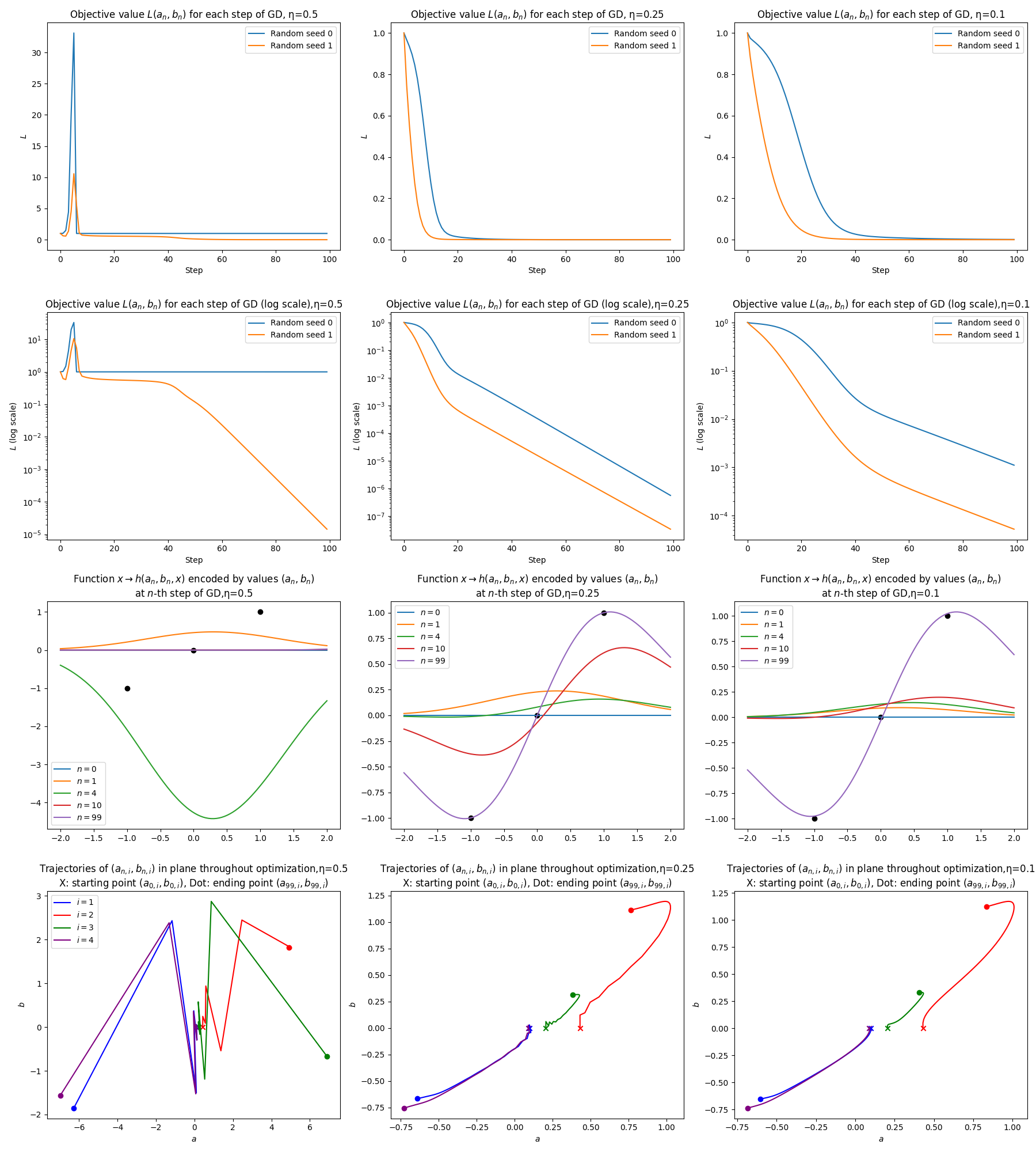
It is up to the user of Algorithm [algo:GD] to pick the parameters \(\eta,N\) under consideration of these trade-offs. Often, one uses the largest \(\eta>0\) that does not lead to numerical errors. For instance, one can first find some step size \(\eta>0\) that does not cause divergence or numerical errors, and then double it until such problems arise (see Figure 3.2).

\(\,\)
Consider the optimization problem \[\text{minimize }L(a,b)\quad\text{for}\quad a,b\in\mathbb{R}^{4},\tag{3.2}\] where \[L(a,b)=\frac{1}{2}\sum_{k=1}^{3}(h(a,b,x_{k})-y_{k})^{2}\] for \[\begin{aligned}
h(a,b,x) & =\sum_{i=1}^{4}g(a_{i},b_{i},x),\qquad a,b\in\mathbb{R}^{4},x\in\mathbb{R},\\
g(a,b,x) & =be^{-\frac{1}{2}(x-a)^{2}},\qquad a,b\in\mathbb{R},x\in\mathbb{R},\tag{3.3}
\end{aligned}\] and \[(x_{1},y_{1})=(-1,-1),\qquad(x_{2},y_{2})=(0,0),\qquad(x_{3},y_{3})=(0,1).\tag{3.4}\] The function \(h(a,b,x)\) represents a parameterized class of scalar functions \[x\to h(a,b,x),\] where \(a,b\in\mathbb{R}^{4}\) are the parameters. The function \(h(a,b,x)\) consists for four superimposed “bump functions” \[x\to g(a_{i},b_{i},x),\] where the parameter \(a_{i}\) specifies the location of the \(i\)-th bump, and \(b_{i}\) is parameter determining the bump functions sign and magnitude (see (3.3)).
For any parameters \(a,b,\) the function \(L(a,b)\) is a measure of how well the parametric function matches three “data points” \((x_{k},y_{k}),k=1,2,3,\) i.e. how good the approximation \[h(a,b,x_{k})\approx y_{k}\] is for those parameter values. Minimizing \(L(a,b)\) over \(a,b\in\mathbb{R}^{4}\) entails optimizing for the best fit of the parametric function \(x\to h(a,b,x)\) to the datapoints.
The parametric function \(h(a,b,x)\) is in fact a simple artificial neural network, and minimizing \(L(a,b)\) is the corresponding learning algorithm. We will study artificial neural networks in the Machine Learning part of the course.
We now apply gradient descent to (approximately) solve the minimization problem (3.2). To do so we must first compute the gradient \(\nabla L(a,b).\) Using the chain rule we have \[\partial_{a_{i}}L(a,b)=\frac{1}{2}\sum_{k=1}^{3}\partial_{a_{i}}\left\{ (h(a,b,x_{k})-y_{k})^{2}\right\} =\sum_{k=1}^{3}(h(a,b,x_{k})-y_{k})\partial_{a_{i}}\{h(a,b,x_{k})\},\] and similarly \[\partial_{b_{i}}L(a,b)=\frac{1}{2}\sum_{k=1}^{3}2(h(a,b,x_{k})-y_{k})\partial_{b_{i}}\{h(a,b,x_{k})\}.\] Furthermore \[\begin{aligned} \partial_{a_{i}}\{h(a,b,x_{k})\} & =\sum_{i=1}^{4}\partial_{a_{i}}\{g(a_{i},b_{i},x)\}=\partial_{a}g(a_{i},b_{i},x),\\ \partial_{b_{i}}\{h(a,b,x_{k})\} & =\partial_{b}g(a_{i},b_{i},x). \end{aligned}\] Lastly \[\begin{aligned} \partial_{a}g(a,b,x) & =b\partial_{a}e^{-\frac{1}{2}(x-a)^{2}}=b(x-a)e^{-\frac{1}{2}x(x-a)^{2}}=(x-a)g(a,b,x),\\ \partial_{b}g(a,b,x) & =e^{-\frac{1}{2}(x-a)^{2}}. \end{aligned}\] Thus \[\begin{aligned} \partial_{a_{i}}L(a,b) & =D_{a,i}(a,b):=\sum_{k=1}^{3}(h(a_{i},b_{i},x_{k})-y_{k})(x_{k}-a_{i})g(a_{i},b_{i},x_{k}),\\ \partial_{b_{i}}L(a,b) & =D_{b,i}(a,b):=\sum_{k=1}^{3}(h(a_{i},b_{i},x_{k})-y_{k})e^{-\frac{1}{2}(x_{k}-a_{i})^{2}}. \end{aligned}\] The iteration of gradient descent then reads \[\begin{aligned} a_{n+1,i} & =a_{n,i}-\eta D_{a,i}(a_{n},b_{n}),\\ b_{n+1,i} & =b_{n,i}-\eta D_{b,i}(a_{n},b_{n}). \end{aligned}\]
Note that if \(a=b=0,\) then \(D_{a,i}(a,b)=0\) regardless of the values of \((x_{k},y_{k}),\) and for these particular \(x_{k},y_{k}\) also \(D_{b,i}(a,b)=0\) by symmetry. Thus if we set \[a_{0}=b_{0}=(0,0,0,0),\] then the iterates of gradient descent will stay fixed at these values forever: \[a_{n}=b_{n}=0\quad\forall n\ge0.\] This clearly not desirable. To avoid this one could set say \[a_{0}=b_{0}=(1,1,1,1).\tag{3.5}\] Then \(D_{a,i}(a_{0},b_{0})\ne0\) and \(D_{b,i}(a_{0},b_{0})\ne0\) for all \(i=1,2,3,4,\) so gradient descent is not stuck at the starting point. But note that if \(a_{0,1}=\ldots=a_{0,4}\) and \(b_{0,1}=\ldots=b_{0,4},\) then \(D_{a,i}(a_{0},b_{0})\) and \(D_{b,i}(a_{0},b_{0})\) take the same value for each \(i.\) Thus each entry of \(a_{n}\) and \(b_{n}\) are identical for every \(n,\) so gradient descent effectively stays stuck inside the subspace where \(a_{1}=\ldots=a_{4},\) \(b_{1}=\ldots=b_{4}.\) The latter is the subspace of functions \(x\to h(a,b,x)\) that effectively have only one “bump” function. A single bump function can not fit the data set (3.4), so the initial condition (3.5) is not suitable.
In such situations it is common to start with random parameter values. For this problem one can for instance initialize \[a_{0,1},\ldots,a_{0,4}\text{ as independent uniform random variables on }[-1,1],\] combined with \[b_{0}=(0,0,0,0).\]
The following is an implementation in python of gradient descent for solving (3.2).
import numpy as np

def g(a,b,x):
    return b*np.exp(-0.5*(x-a)**2)

# Gradient of g wrt to a
def grad_g_a(a,b,x):
    return (x-a)*g(a,b,x)

# Gradient of g wrt to b
def grad_g_b(a,b,x):
    return np.exp(-0.5*(x-a)**2)

def h(avec,bvec,x):
    ret = 0
    for i in range(len(avec)):
        ret += g(avec[i],bvec[i],x)
    return ret

# Gradient of h
def grad_h(avec,bvec,x):
    reta = np.zeros(len(avec))
    retb = np.zeros(len(bvec))
    for i in range(len(avec)):
        reta[i] = grad_g_a(avec[i],bvec[i],x)
        retb[i] = grad_g_b(avec[i],bvec[i],x)
    return (reta,retb)

def L(avec,bvec,xvec,yvec):
    ret = 0
    for k in range(len(xvec)):
        ret += (h(avec,bvec,xvec[k])-yvec[k])**2/2.0
    return ret

# Gradient of L
def grad_L(avec,bvec,xvec,yvec):
    reta = np.zeros(len(avec))
    retb = np.zeros(len(bvec))
    for k in range(len(xvec)):
        (ga,gb) = grad_h(avec,bvec,xvec[k])
        reta += (h(avec,bvec,xvec[k])-yvec[k])*ga
        retb += (h(avec,bvec,xvec[k])-yvec[k])*gb
    return (reta,retb)

# Run GD starting from avec, bvec
def GD_minimize(avec,bvec,xvec,yvec,num_steps):
    histL = []
    hista = []
    histb = []

    for n in range(num_steps):
        hista.append( avec )
        histb.append( bvec )
        histL.append( L(avec,bvec,xvec,yvec) )
        (ga,gb) = grad_L(avec, bvec, xvec, yvec )
        avec = avec - eta*ga
        bvec = bvec - eta*gb

    return (histL,hista,histb)

# Data points
xvec = np.array( [-1,0,1] )
yvec = xvec

num_bumps = 4
# Initialize parameters
# a initialized randomly
avec0 = np.random.uniform( -1, 1, num_bumps )
# b initialized as zerobvec0 = np.zeros( num_bumps )

num_steps = 100 # Number of steps of GD
eta = 0.1 # Step-size

# Run GD
(histL,hista,histb) = GD_minimize(avec0,bvec0, \
                                 xvec,yvec,num_steps)
See Section 3.8 for additional code examples for debugging gradient calculations, and for producing plots based on the results of the above code.
The results of running this code with different values of \(\eta\) is shown in Figure 3.6.
Even if gradient descent is numerically stable and converges, there is no guarantee that the algorithm results in a good approximation of a global minimizer of the objective function \(f.\) Indeed, one can hope for such a guarantee only if \(f\) is convex. It is easy to convince oneself of this from the following diagrams for the case \(d=1.\)

For the non-convex \(f\) plotted on the top row of Figure 3.4, gradient descent can converge to a non-global local minimum, or diverge to \(\infty\) without achieving the global minimum, if started in the corresponding “regions of attraction”. There is also a “region of attraction” for the global minimum. For dimension \(d=1\) (and sometimes \(d=2\)) one can easily visualize the objective function and work out what kind of behavior to expect from gradient descent. For high-dimensional (\(d\) large) non-convex functions it is in general very hard to reach the same level of understanding. However, it should be noted that gradient descent is often applied to high-dimensional non-convex problems with good results. In those settings, the vector \(x_{N}\) returned by gradient descent turns out to be good in some sense specific to the problem being solved - one just lacks guarantees that there aren’t better \(x\) that gradient descent missed.