8 Condition Number of Matrices
We would like to assign a condition number to a matrix \(A\) in order to quantify whether the linear system represented by \(A\) is well- or ill-conditioned. This requires some preparations, as the condition number was based on measuring distances, i.e. on the absolute value in \(\mathbb{R}.\) We now generalize the concept of absolute value to \(\mathbb{R}^n.\)
8.1 Euclidean Norm
As we have equipped the real numbers with the absolute value \(|\cdot|,\) we can equip \(\mathbb{R}^n\) with a measure for length and distances.
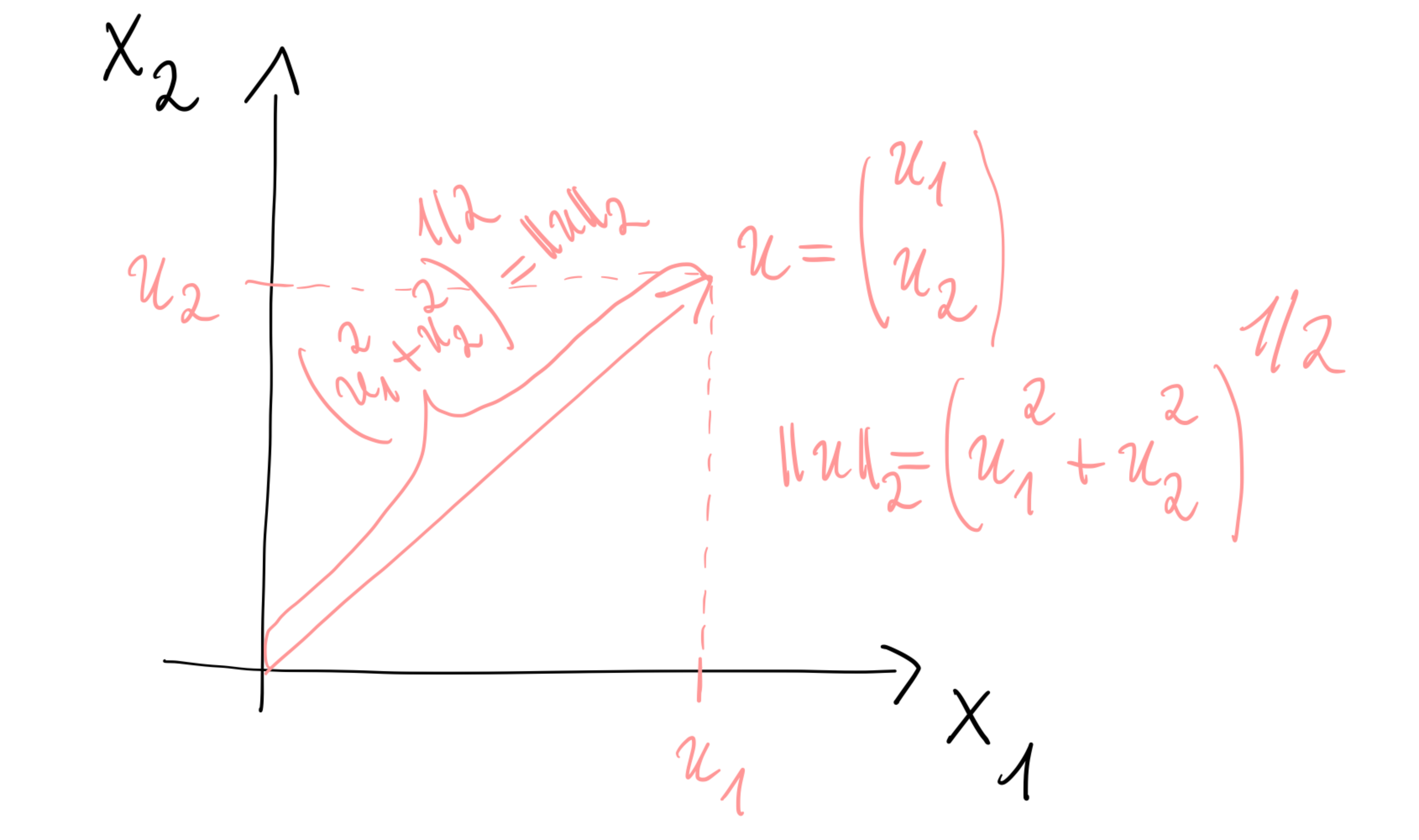
The most common measure for length and distance is the Euclidean norm \[\|x\|_2 = \left(\sum_{i=0}^n x_i^2 \right)^{1/2}, \qquad x=\begin{pmatrix}x_1\\ \vdots\\x_n\end{pmatrix}\in \mathbb{R}^n\, .\] Figure 8.1 illustrates the Euclidean norm in \(\mathbb{R}^2\) and shows that its definition is based on the theorem of Pythagoras.
In many respects, the Euclidean norm behaves similarly to the absolute value. Theorem 8.1 below generalizes Theorem 1.1 from \(\mathbb{R}\) to \(\mathbb{R}^n.\)
Theorem 8.1
Let \(\|\cdot\|_2: X\to\mathbb{R}_0^+\) be the Euclidean norm. Then, \(\|\cdot\|_2\) has the following properties:
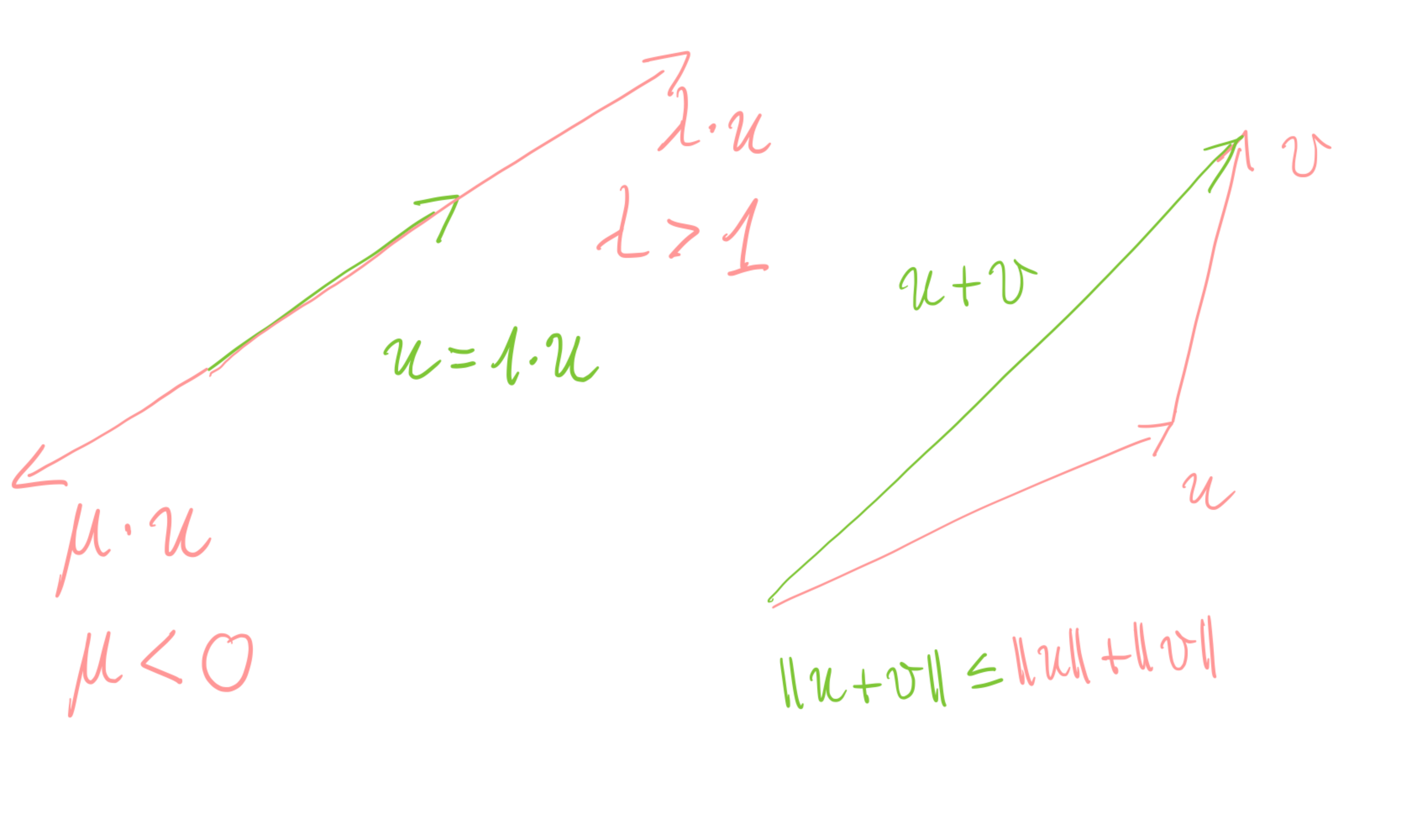
\(\|x\|_2=0\iff x=0,\)(definiteness)
\(\|\lambda x\|=|\lambda|\|x\|_2\quad\text{for all } x\in X,\lambda\in\mathbb{R},\) (homogeneity)
\(\|x+y\|_2\le \|x\|_2 + \|y\|_2 \quad\text{for all } x,y\in X.\) (triangle inequality)
As we have seen above, the Euclidean space \(\mathbb{R}^n\) can be equipped with the Euclidean norm \(\|\cdot\|_2,\) which introduces the capability to measure the “length” \(\|x\|\) of a vector \(x\in\mathbb{R}^n\) as well as the distance \(\|x-y\|\) between two vectors \(x,y\in\mathbb{R}^n\)
8.1.1 Some norms
As can be shown, \(\|\cdot\|_2\) is not the only norm on \(\mathbb{R}^n.\) In fact, different choices for norms, i.e. mappings which have the properties of Theorem 8.1, are possible. For example, for each \(p\ge 1,\) we can define the \(p\)-norm of the vector \(x\) by \[{\left\|{x}\right\|}_{{p}}=\left(\sum\limits_{i=1}^n|x_i|^p\right)^{1/p}\, .\] For \(p=2\) we get the Euclidean norm back, which therefore is also often referred to as the \(2\)-norm.
As an additional example, the infinity-norm is defined by \[{\left\|{x}\right\|}_{{\infty}}=\max\limits_{i=1,\ldots, n}|x_i| \, .\]
8.1.2 The Unit Ball
In order to visualize the differences between the above norms, we first make a definition:
Definition 8.1
Let \(\delta >0\) be a real number and \(x\in\mathbb{R}^n.\) Then we call the set \[B_{\delta}(x) =\{z\in \mathbb{R}^n \colon \|z-x\| < \delta\}\, .\] the (open) ball with radius \(\delta\) around \(x\) (w.r.t. the norm \(\|\cdot\|\)).
The (open) unit ball \((X, \|\cdot\|)\) is defined as \[B_{1}(0) =\{z\in \mathbb{R}^n \colon \|z\| < 1\}\, .\]
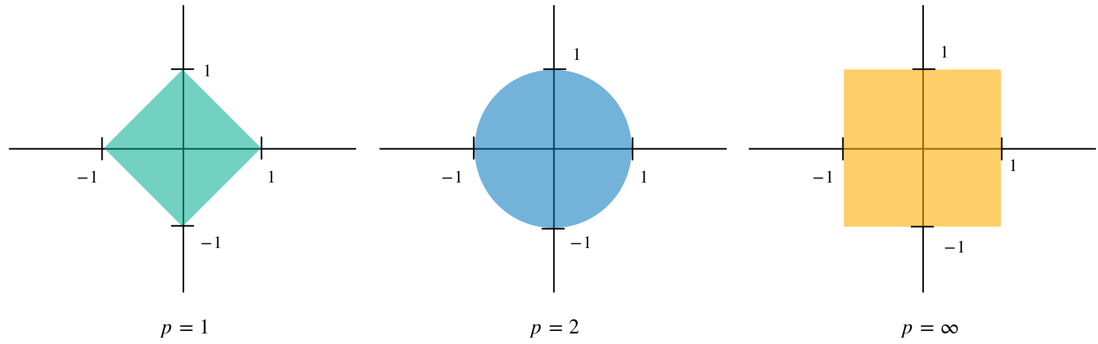
Plotting the unit ball in \(X=\mathbb{R}^2\) for different norms is very helpful for understanding the differences between norms and developing a visual understanding.
Figure 8.3 shows the unit ball in \(\mathbb{R}^2\) for the \(p\)-norm with \(p=1,2,\infty.\)
8.2 Condition Number of Matrices
8.2.1 Absolute Condition
We recall the definition (5.1) of the constant \(L_{\mathrm{abs}}\) \[|f(x)- f(\tilde{x})| \leq L_{\mathrm{abs}} |x-\tilde{x}|\, ,\] \(x,\tilde{x}\in X,\) which we have used for defining the (absolute) condition number of a problem. We simply replace the absolute value in this equation by a norm and insert \(f(x) = Ax,\) where \(A\in \mathbb{R}^{n\times n}\) is a matrix, and arrive at \[\tag{8.2} \begin{aligned} \|Ax- A\tilde{x}\| &\leq L_{\mathrm{abs}} \|x-\tilde{x}\|\, . \end{aligned}\] Due to the linearity of the matrix-vector product, we have \(Ax- A\tilde{x}=A(x- \tilde{x})\) and obtain \[\begin{aligned} \|Ax- A\tilde{x}\| &=\|A(x- \tilde{x})\|\\ &\leq L_{\mathrm{abs}} \|x-\tilde{x}\|\,, \end{aligned}\] or, as \(x\not =\tilde{x},\) \[\begin{aligned} \frac{\|A(x- \tilde{x})\|}{\|x-\tilde{x}\|} &\leq L_{\mathrm{abs}} \,. \end{aligned}\] Setting now \(y=x-\tilde{x}\not= 0,\) we see that \(L_{\mathrm{abs}}\) can be characterised as the smallest constant with \[\begin{aligned} \frac{\|Ay\|}{\|y\|} &\leq L_{\mathrm{abs}} \end{aligned}\] for \(0\not =y\in\mathbb{R}^n.\) Thus, the absolute condition of \(A\in\mathbb{R}^{n\times n}\) can be computed as —if the supremum exists— \[L_{\mathrm{abs}} = \sup_{0\not =y\in\mathbb{R}^n} \frac{\|Ay\|}{\|y\|}\, .\]
8.2.2 Matrix Norm
We turn our above considerations into a definition:
Definition 8.2
Let \(A\in\mathbb{R}^{n\times n}\) be a matrix. We call \[\tag{8.3} \begin{aligned} \|A\| &= \max_{x\not = 0} \frac{\|Ax\|}{\|x\|}\\ &= \max_{\|x\|= 1} \|Ax\| \end{aligned}\] the matrix norm of \(A.\)
In order to better understand the above definition, we investigate the matrix norm of \(A\) —or the absolute condition of \(A\)— in more detail. First, we see that \[\|I\| = \max_{\|x\|= 1} \|Ix\| = \max_{\|x\|= 1} \|x\| =1\] for any matrix norm.
Second, we see that from the definition we get for any \(0\not = x\in\mathbb{R}^n\) \[\begin{aligned} \frac{\|Ax\|}{\|x\|} &\leq \max_{x\not = 0} \frac{\|Ax\|}{\|x\|}\\ &= \|A\|\, , \end{aligned}\] which after multiplication with \(\|x\|\) gives rise to \[\tag{8.4} \begin{aligned} \|Ax\| &\leq \|A\| \|x\|\, . \end{aligned}\] Since for \(x=0\) Equation (8.4) simply reads \(0\leq 0,\) we see that (8.4) holds for all \(x\in\mathbb{R}^n.\)
Third, we see that the matrix norm can be interpreted as the maximal distortion of the unit ball when \(A\) is applied. For example, let us consider the case of a diagonal matrix \(D=\mathop{\mathrm{diag}}(d_1, \ldots ,d_n)\) with \(d_i\neq0\) for \(i=1, \ldots ,n.\) We see that \(D\) simply scales coordinate direction \(i\) with the factor \(d_i.\) Thus, in two dimensions, i.e. \(n=2,\) the unit ball —or unit circle— of the Euclidean norm is mapped to an ellipsoid. The maximal distortion is \[\|D\| = \max_{i=1,\ldots,n} |d_i|\, .\]
Exercise 8.1
Prove the above statement.
Theorem 8.2 • Submultiplicativity of the Matrix Norm
Let \(A,B\in\mathbb{R}^{n\times n}\) be two matrices. It holds \[\tag{8.5} \begin{aligned} \|AB\| &\leq \|A\|\|B\|\, . \end{aligned}\] We say that the matrix norm is submultiplicative.
Proof. Exercise.
8.2.3 Relative Condition: Condition Number of a Matrix
Looking at the relative condition number of the linear mapping represented by the invertible matrix \(A\in\mathbb{R}^{n\times n},\) we arrive for \(x\not =\tilde{x}\) and \(x\not = 0\) at, \[\begin{aligned} \frac{\|Ax - A\tilde{x}\|}{\|Ax\|} &\leq L_{\mathrm{rel}} \frac{\|x- \tilde{x}\|}{\|x\|} \end{aligned}\] or \[\begin{aligned} \frac{\|A(x - \tilde{x})\|}{\|Ax\|} &\leq L_{\mathrm{rel}} \frac{\|x- \tilde{x}\|}{\|x\|}\, . \end{aligned}\] We can immediately estimate \[\begin{aligned} \frac{\|A(x - \tilde{x})\|}{\|Ax\|} & \leq \|A\| \frac{\|x- \tilde{x}\|}{\|Ax\|} \\ &= \|A\|\frac{\|x\|}{\|Ax\|}\frac{\|x- \tilde{x}\|}{\|x\|} \, . \end{aligned}\] We now observe that for invertible \(A\) we have \[\|A^{-1}\| = \max_{\mathbb{R}^n\ni x\not=0} \frac{\|A^{-1}x\|}{\|x\|} = \max_{\mathbb{R}^n\ni y=A^{-1}x\not=0} \frac{\|y\|}{\|Ay\|}\, .\] We can use this to estimate the term \(\frac{\|x\|}{\|Ax\|}\) and get \[\begin{aligned} \frac{\|Ax - A\tilde{x}\|}{\|Ax\|} &\leq \|A\|\frac{ \|x\|}{\|Ax\|}\frac{\|x- \tilde{x}\|}{\|x\|} \\ &\leq \|A\|\|A^{-1}\| \frac{\|x- \tilde{x}\|}{\|x\|}\,, \end{aligned}\] or \(L_{\mathrm{rel}} = \|A\|\|A^{-1}\|.\) This motivates the following
Definition 8.3 • Condition Number for invertible Matrices
Let \(A\in\mathbb{R}^{n\times n}\) be an invertible matrix. We call \[\tag{8.6} \begin{aligned} \kappa(A) = \|A\|\cdot \|A^{-1}\| \end{aligned}\] the (relative) condition number of \(A.\)
Clearly, we have \(\kappa(A) = \kappa (A^{-1}).\) The condition number is always larger or equal to one for invertible matrices: \[1=\|I_n\|= \|A A^{-1}\| \leq \|A\| \|A^{-1}\| = \kappa(A)\, .\] Moreover, the condition number is invariant to scaling with a scalar \(0\not =\alpha\in\mathbb{R}\) \[\kappa(A) = \kappa(\alpha A)\, .\] We eventually note that for \(A\) not invertible we set \[\tag{8.7} \kappa(A) = \frac{\max_{x\not = 0}\frac{\|Ax\|}{\|x\|}}{\min_{x\not = 0}\frac{\|Ax\|}{\|x\|}}\, .\]
As an application of (8.6), we consider for \(b\in \mathbb{R}^n\) and invertible \(A\in\mathbb{R}^{n\times n}\) the linear system \[Ax=b\, .\] Let \(\tilde{x}\not = x\) be an approximate solution of this linear system, leading to the residual \[r = b- A\tilde{x} = A(x-\tilde{x})\, ,\] Then, we see that the relative error of \(\tilde{x}\) can be estimated as \[\begin{aligned} \frac{\|x-\tilde{x}\|}{\|x\|} &= \frac{\|A^{-1} (b-A\tilde{x})\|}{\|A^{-1} b\|}\\ &\leq \kappa(A) \frac{\|b-A\tilde{x}\|}{\|b\|} \, . \end{aligned}\] We see from this estimate that the (relative) error of the residual is only a reliable estimate for the true (relative) error \(x-\tilde{x}\) within the limits of the condition number. In other words:
Remark 8.1
The (relative) distance to the singular matrix closest to \(A\) (measured in your matrix norm) is given by \(\frac{1}{\kappa(A)}.\) The larger the condition number, the closer you are to the set of singular matrices! As we do our computations in a floating point system, at a certain point your matrix \(A\) and a close-to-singular matrix will become indistinguishable. Thus, we call a matrix with \(\kappa(A) \geq \text{eps}\) numerically singular, as its relative distance to the set of non-invertible matrices is smaller than the machine accuracy.
Remark 8.2
Consider the 2-norm of a matrix. Practically speaking, you can use “norm" or “cond" in Matlab. The computation itself is usually done by means of a numerical method, which is called “Singular Value Decomposition" or “svd" in short. You will learn about this method in the Numerics module. As this method requires certain knowledge of linear algebra, it is not part of our introductory module. To motivate the underlying idea, you might want to have a look at the maximum we have to compute (in the following, \(\| \cdot \| = \| \cdot \|_2 = \langle \cdot, \cdot \rangle^{\frac{1}{2}}\)). We have \[\|A\| = \max_{\|x\| = 1} \|Ax\| = \max_{x \neq 0} \frac{\langle Ax, Ax \rangle^{\frac{1}{2}}}{\langle x, x \rangle^{\frac{1}{2}}} = \max_{x \neq 0} \frac{\langle A^TAx, x \rangle^{\frac{1}{2}}}{\langle x, x \rangle^{\frac{1}{2}}}.\] As you know, if \(A\) is regular, then \(A^TA\) is symmetric positive definite (s.p.d.). You will learn in linear algebra that for any s.p.d. matrix \(B \in \mathbb{R}^{n, n},\) there exists a basis of pairwise orthogonal vectors \(\{v_1, \ldots, v_n\}\) which all have norm 1, i.e. we have \(\|v_i\| = 1\) for \(i = 1, \ldots, n,\) and which all are so-called “eigenvectors", i.e. we have \(Bv_i = \lambda_i v_i\) for \(i = 1, \ldots, n\) for some real \(\lambda_i > 0.\) Consequently, every \(x \in \mathbb{R}^n\) can be written as \(x = \sum_{i=1}^n \alpha_i v_i\) with some coefficients \(\alpha_i \in \mathbb{R}\) and we furthermore have \[Bx = B(\sum_{i=1}^n \alpha_i v_i) = \sum_{i=1}^n B(\alpha_i v_i) = \sum_{i=1}^n \lambda_i \alpha_i v_i,\] and furthermore (please do the calculation yourself, you have to exploit orthogonality and the fact that \(\|v_i\| = 1\)) we get \[\langle Bx, x \rangle = \sum_{i=1}^n \lambda_i \alpha_i^2.\] As all \(\lambda_i\) are positive, we can estimate \(\langle Bx, x \rangle \leq \lambda_{\max}(B) \sum_{i=1}^n \alpha_i^2,\) where \(\lambda_{\max}(B)\) is the maximal eigenvalue of \(B.\) If we apply this to \(A^TA = B\) with \(x\) as above, we see that \[\max_{x \neq 0} \frac{\langle A^TAx, x\rangle^{\frac{1}{2}}}{\langle x, x\rangle^{\frac{1}{2}}} \leq \max_{x \neq 0} \frac{\lambda_{\max}(A^TA)^{\frac{1}{2}} \sum_{i=1}^n \alpha_i^2}{\sum_{i=1}^n \alpha_i^2} = \lambda_{\max}(A^TA)^{\frac{1}{2}}.\] The values \(\lambda_i (A^TA)^{\frac{1}{2}}\) are called “singular values" of \(A.\) You can compute them in Matlab using the command “svd". A similar argument applied to the norm of the inverse will lead you to the smallest singular value, which then allows you to compute the 2-norm of a matrix. As pointed out above, this will be done in detail in the Numerics module later on.
8.3 Stability Analysis of Gaussian Elimination
Stability analysis of Gaussian elimination is an optional topic. However, readers are encouraged to read through this material.
Using the concept of matrix norms we have introduced above, we can now analyse in more detail what happens inside the Gaussian elimination.
For a reduction of the considerations below to the case \(n=3,\) we refer to the videos of the Voluntary Material — Stability of Gaussian Elimination.
Theorem 8.3
Let \(A=LU\) and let \[\left( \prod\limits_{i>j}N_{ij}(-l_{ij})\right) = \text{I}-G_j\, ,\] where \(N_{ij}(-l_{ij})\) are the transformation matrices generated during the computation of the decomposition, i.e. \(R=(I-G_{n-1})\cdots(I-G_1)A.\) Then we have \[\kappa(R)\le\prod\limits_{k=1}^{n-1}\kappa(I-G_k)\kappa(A).\]
Proof. We have \[{\left\|{R}\right\|}_{{}}={\left\|{(I-G_k)\cdots(I-G_1)A}\right\|}_{{}} \le\prod\limits_{k=1}^{n-1}{\left\|{I-G_k}\right\|}_{{}}{\left\|{A}\right\|}_{{}}.\] Furthermore, \[{\left\|{R^{-1}}\right\|}_{{}}={\left\|{A^{-1}(I-G_1)^{-1}\cdots(I-G_{n-1})^{-1}}\right\|}_{{}} \le\prod\limits_{k=1}^{n-1}{\left\|{(I-G_k)^{-1}}\right\|}_{{}}{\left\|{A^{-1}}\right\|}_{{}}.\] This implies \[\kappa(R)=\|R\|\|R^{-1}\| \le\prod\limits_{k=1}^{n-1}\|I-G_k\|\|(I-G_k)^{-1}\| \|A\| \|A^{-1}\| = \prod\limits_{k=1}^{n-1}\kappa(I-G_k)\kappa(A).\]
Note 8.1
\[\kappa(R)=\prod\limits_{k=1}^{n-1}\kappa(I-G_k)\kappa(A)\ge\kappa(A).\] LU-decomposition enlarges the error by the factor \[\prod\limits_{k=1}^{n-1}\kappa(I-G_k).\]
Note 8.2
A pathological example: Wilkinson-Matrix Let \[A=(a_{ij})_{1\leq i,j \leq n}= \begin{cases} 1&\text{ if }i=j,\ j=n,\\ -1&\text{ if }i>j,\\ 0&\text{ else. } \end{cases} =\begin{pmatrix} 1 & & & &1\\ -1 &\ddots& 0 & &\vdots\\ \vdots&\ddots&\ddots& &\vdots\\ \vdots& &\ddots&\ddots&\vdots\\ -1 &\cdots&\cdots&-1&1 \end{pmatrix}.\] Then we have for \(n=50\): \(\kappa(A)=22.3\) and \(\kappa(U)=7.5\cdot10^{14}.\) This implies instability of the LU-decomposition for this matrix.
Theorem 8.4
We have \[\kappa_{\infty}(I-G_k)=(1+\max\limits_{i=k+1, \ldots ,n}|l_{ij}|)^2.\]
Proof. \({\left\|{\cdot}\right\|}_{{\infty}}\) is the row-sum norm. Thus, we have \[{\left\|{I-G_k}\right\|}_{{\infty}}=1+\max\limits_{i=k+1, \ldots ,n}|l_{ik}|\] and \((I-G_k)^{-1}=I+G_k\) \((N_{ij}(-\alpha)=N_{ij}(\alpha)^{-1})\) implies \[{\left\|{(I-G_k)^{-1}}\right\|}_{{\infty}}={\left\|{1+G_k}\right\|}_{{\infty}} =1+\max\limits_{i=k+1, \ldots ,n}|l_{ik}|.\] Now, by definition we have \[\kappa_\infty(I-G_k)={\left\|{I-G_k}\right\|}_{{\infty}}{\left\|{I+G_k}\right\|}_{{\infty}} =(1+\max\limits_{i=k+1, \ldots ,n} |l_{ik}|)^2\, .\]
As a consequence, \(\kappa(I-G_k)>1\) and \(\max_{i=k+1, \ldots ,n}|l_{ik}|\gg 1\) imply a (potential) instability of the LU-decomposition. Ideally, we would have a pivoting strategy leading to a pivoting index \(p'\) with \[\max\limits_{i=j, \ldots ,n}\frac{|a_{ij}^{(j-1)}|}{|a_{pj}^{(j-1)}|} \le\max\limits_{i=j, \ldots ,n}\frac{|a_{il}^{(j-1)}|}{|a_{p' l}^{(j-1)}|} \quad\text{ for all }l=j, \ldots ,n\, .\] However, this is computationally too expensive. An alternative is Scaling.
Note 8.3
\[\begin{pmatrix}1&0\\0&\epsilon\end{pmatrix}\leadsto \begin{pmatrix}1&0\\0&1\end{pmatrix}.\]
There are some variants:
Equilibration of rows w.r.t. \({\left\|{\cdot}\right\|}_{{}}\): Scale row \(j\) with \({\left\|{A^j}\right\|}_{{}}^{-1},\) where \(A^j\) denotes row \(j\) of \(A.\)
Equilibration of columns w.r.t \({\left\|{\cdot}\right\|}_{{}}\): Scale the \(j\)-th column \(A_j\) with \({\left\|{A_j}\right\|}_{{}}^{-1}.\)
Complete equilibration (rows and columns): Due to the non-linearity of the norm this leads in general to a non-linear system in \(2n-2\) variables. This is not only computationally too expensive but also contains a scaling problem. Thus, in most linear algebra libraries, the user is asked to provide an appropriate scaling if required.
8.3.0.0.1 Iterative Refinement
We want to solve the linear system \(Ax=b.\) By LU-decomposition we have obtained \(x_0'\) with residual \(b-A x_0'\neq 0.\) From \(b=Ax\) we have \(b-Ax_0'=A(x-x'_0)\) and with \(A\Delta x_0'=b-Ax_0'\) we would get \[A(x_0'+\Delta x_0')=Ax_0'+b-A x_0'=b \, .\] The process \(x_0'\mapsto x_1'= x_0'+\Delta x_0'\) is called iterative refinement. Iterative refinement requires \(\mbox{\large$\mathcal{O}$}(n^2)\) operations. AXXBT4G1LW49PVMSAKZCQJVITZOSNORP
9 Symmetry, Cholesky Decomposition, and Rank
9.1 Scalar Product
We now consider the Euclidean scalar product, which will help us to understand concepts such as orthogonality. Let us recall the definition of the Euclidean norm \[\|x\|_2 = \left(\sum_{i=1}^n x_i^2 \right)^{1/2}, \qquad x=\begin{pmatrix}x_1\\ \vdots\\x_n\end{pmatrix}\in \mathbb{R}^n\, .\]
Definition 9.1
We define the Euclidean scalar product \[\begin{aligned} \langle\cdot,\cdot\rangle \colon\mathbb{R}^n\times\mathbb{R}^n\longrightarrow \mathbb{R}\\ \langle x, y \rangle = \sum_{i=1}^n x_i y_i\, . \end{aligned}\]
Furthermore, the Euclidean scalar product has the following properties:
\(\langle x,y\rangle= \langle y,x\rangle\) for all \(x,y\in\mathbb{R}^n\) (symmetric)
\(\langle x,x\rangle > 0\) for all \(x\in\mathbb{R}^n\) with \(x\neq0\) (positive definite)
\(\langle \alpha x+\beta y,z\rangle=\alpha\langle x,z\rangle +\beta \langle y,z\rangle\) for all \(\alpha,\beta\in\mathbb{R}\) and all \(x,y,z\in\mathbb{R}^n\) (bi-linear form)
Proof. Exercise.
We see that for \(x\in\mathbb{R}^n\) we have \[\tag{9.1} \|x\| = \langle x,x\rangle^{1/2}\, .\]
We will now see that \(\langle\cdot,\cdot\rangle\) creates a geometry on \(\mathbb{R}^n.\) We start with the important Cauchy-Schwarz inequality.
Theorem 9.1 • Inequality of Cauchy-Schwarz
Let \(u,v\in \mathbb{R}^n.\) Then it holds \[\tag{9.2} |\langle u,v\rangle |\le{\left\|{u}\right\|}_{{2}}{\left\|{v}\right\|}_{{2}} \, .\]
An immediate consequence of this inequality is the following
Corollary 9.2
We have \[\tag{9.3} \frac{\langle u,v\rangle }{{\left\|{u}\right\|}_{{2}}{\left\|{v}\right\|}_{{2}}}\in[-1,1]\, .\]
The above estimate (9.3) allows us to interpret the expression \(\frac{\langle u,v\rangle }{{\left\|{u}\right\|}_{{2}}{\left\|{v}\right\|}_{{2}}}\) as the cosine of the angle between two vectors \(0\neq u,v\in \mathbb{R}^n.\) We can set \[\tag{9.4} \cos\angle(u,v)=\frac{\langle u,v\rangle}{{\left\|{u}\right\|}_{{2}}{\left\|{v}\right\|}_{{2}}}\, .\] Exploiting this definition, we call two vectors perpendicular, or orthogonal, if \[\langle u,v\rangle =0,\] and write \(u\perp v.\) Clearly, if \(u\) and \(v\) are orthogonal, inequality (9.2) will, in general, not be sharp, as the left-hand side \(|\langle u,v\rangle|\) will be zero and the right-hand side \({\left\|{u}\right\|}_{{2}}{\left\|{v}\right\|}_{{2}}\) can become arbitrarily large, depending on \(u,v.\) We now ask ourselves: Under which circumstances will inequality (9.2) be sharp, i.e. when will \[|\langle u,v\rangle |={\left\|{u}\right\|}_{{2}}{\left\|{v}\right\|}_{{2}}\] hold? Left as an exercise for the reader.
9.2 Cholesky-Decomposition
The \(LU\)–decomposition can be simplified for matrices with a special structure, namely, the so-called symmetric potitive definite (spd) matrices.
We start with the definition of a symmetric positive definite matrix:
We recall that the matrix \(A\in\mathbb{R}^{n \times n}\) is called symmetric if \(A^T=A.\)
Definition 9.2
Let \(A\in\mathbb{R}^{n \times n}\) be a matrix. We call \(A\) positive definite if \[\tag{9.5} \langle x,Ax\rangle > 0 \quad\text{ for all }x\in\mathbb{R}^n, \quad x\neq 0\, .\] We call \(A\) symmetric positive definite (spd) if \(A\) is symmetric and positive definite.
Remark 9.1
The expression \[x^TAx=\langle x,Ax\rangle =\sum\limits_{i,j=1}^n x_i a_{ij} x_j =\sum\limits_{i=1}^n x_i^2 a_{ii} + \sum\limits_{\genfrac{}{}{0pt}{}{\scriptstyle i,j=1}{\scriptstyle i\neq j}}^n x_i a_{ij} x_j\] is called a quadratic form.
We investigate the properties of symmetric positive definite matrices.
Theorem 9.3
Let \(A\in\mathbb{R}^{n\times n}\) be symmetric positive definite. Then we have:
\(A\) is invertible;
\(a_{ii}>0\) for \(i=1, \ldots ,n\);
\(\max\limits_{i,j} |a_{ij}|=\max\limits_i a_{ii}.\)
Proof.
Let us assume that \(A\) would not be invertible. Then, there would exist an \(x\neq0\in\mathbb{R}^n\) with \(Ax=0.\) This would imply \(\langle x,Ax\rangle =0\) for \(x\neq0,\) i.e. \(A\) would not be positive definite.
Let \(e_i\) be the \(i\)-th canonical unit-vector of \(\mathbb{R}^n.\) Then we have \(\langle e_i,Ae_i\rangle =a_{ii}>0,\) since \(A\) is positive definite.
From \[0 < \langle e_i+e_j,A(e_i+e_j) \rangle=\langle e_i,Ae_i\rangle +2\langle e_i,Ae_j\rangle +\langle e_j,Ae_j\rangle =a_{ii}+2a_{ij}+a_{jj}\] we get \(-2a_{ij}<a_{ii}+a_{jj}.\) Similarly, \(0<\langle e_i-e_j,A(e_i-e_j)\rangle\) implies \(2a_{ij}\le a_{ii}+a_{jj}.\) Putting everything together, we see \[2\max\limits_{i,j=1, \ldots ,n} |a_{ij}|\le\max\limits_{i,j=1, \ldots ,n}(a_{ii}+a_{jj}) =2\max\limits_{i=1, \ldots ,n}a_{ii}\, ,\] which concludes the proof.
Remark 9.2
(a) Inserting a “particularly selected” vector \(v\) into the form \(\langle \cdot,A\cdot\rangle\) is also called “testing” and \(v\) is called a “test vector”.
(b) Result (iii) in Theorem 9.3 is relevant for pivoting strategies for spd matrices (see the assignment).
Theorem 9.4
Let \(A\in\mathbb{R}^{n\times n}\) be symmetric positive definite. Then, there exists a unique decomposition of the form \[\tag{9.7} A=LDL^T\] where \(L\) is a lower triangular matrix and \(l_{ii} = 1,\) \(i=1, \ldots ,n,\) and \(D\) is a diagonal matrix with strictly positive entries.
As \(D=\mathop{\mathrm{diag}}(d_1, \ldots ,d_n)\) is positive, we can set \(D^{1/2}:=\mathop{\mathrm{diag}}(\sqrt{d_1}, \ldots ,\sqrt{d_n})\) and we see \(A=\overline{L}\overline{L}^T\) with \(\overline{L}:=LD^{1/2}.\) We call \(A=LDL^T\) rational Cholesky decompositon, as it can be computed without taking square roots.
\(\overline{L}\) can be determined by means of the Cholesky decomposition:
for \(j=1, \ldots ,n\)
\(l_{jj}=(a_{jj}-\sum\limits_{k=1}^{j-1}l_{jk}^2)^{1/2};\)
for \(i=j+1, \ldots ,n\)
\(l_{ij}=(a_{ij}-\sum\limits_{k=1}^{j-1}l_{ik}l_{jk})/l_{jj}.\)
This requires approximately \(\frac 16 n^3\) operations and \(n\) square roots as well as \(\frac13n^3\) operations with additions. In contrast, the \(LU\)-decomposition needs about \(\frac 13 n^3\) point operations and \(\frac 23n^3\) operations with additions. That is, the Cholesky decomposition requires roughly half of the computational effort of an \(LU\) decomposition. Furthermore, pivoting is significantly easier.
9.3 Rank of a Matrix
We have considered up to now the case in which the matrix \(A\in\mathbb{R}^{n\times n}\) was invertible. But what happens if \(A\) is not invertible? Again, the answer is given by Gaussian elimination.
9.3.1 Row Echelon Form
Definition 9.3 • Row Echelon Form
(i) Let \(v\in\mathbb{R}^{1 \times n}\) be a row vector. We denote by \(N(v)\) the number of leading zeros of \(v.\) For \(0\leq i\leq n,\) we have \(N(v)=i,\) iff \[v_1=\cdots=v_i=0\, ,\quad v_{i+1}\neq 0\, .\] We set \(N(v)=n\) and \(N(v)=0,\) if \(v_1\neq 0.\)
(ii) Let \(A\in\mathbb{R}^{m \times n}\) and let \(R_i\) denote the \(i\)-th row of \(A.\) We say that \(A\) is in row echelon form if, for \(i\leq m-1,\) we have \[N(R_{i+1})\geq N(R_i) \text{ and } N(R_{i+1}) > N(R_i) \text{ unless } R_i=0\, .\]
We give some examples: \[\begin{pmatrix} 0 & 1 & 0 & 2\\ 0 & 0 & 1 & 3\\ 0 & 0 & 0 & 0\\ \end{pmatrix}\qquad \begin{pmatrix} 1 & 0 & 0 \\ 0 & 1 & 2\\ 0 & 0 & 1\\ \end{pmatrix}\] Gaussian elimination, therefore, is a process which transforms a matrix \(A\) into row-echelon form, i.e. \[\begin{pmatrix} * & & \\ 0 & * & \\ 0 & 0 & *\\ \end{pmatrix}\, ,\] with \(*\) the non-zero pivot elements or pivots. If \(R_i=0\) occurs during Gaussian elimination such that there does not exist an \(R_j\) such that \(R_{ji}\neq0,\) the elimination process stops.
Definition 9.4 • Rank of a Matrix
We call the number \(r\) of pivot elements the rank of the matrix \(A\in\mathbb{R}^{m\times n}\) and write \(r=\mathrm{rank}(A)\) .
As a consequence of the above definition, we see that a quadratic matrix \(A\in\mathbb{R}^{n\times n}\) is invertible iff \(\mathrm{rank}(A) = n.\)
9.3.2 Solution Space and Kernel
We would like to better understand the case of a matrix which does not have full rank. To this end, we consider the linear system \(Ax=b\) with \(A\in\mathbb{R}^{m\times n}.\) For further reference, we make the following definitions
Definition 9.5
(i) We call \[\tag{9.8} \mathrm{Sol}(A,b) =\{x\,|\,x\in\mathbb{R}^n, Ax=b\}\] the solution space of \(A\) and \(b.\)
(ii) We call \[\tag{9.9} \mathrm{ker}(A) =\{x\,|\,x\in\mathbb{R}^n, Ax=0\}\] the kernel of the matrix \(A.\)
Let us now consider the extended coefficient matrix once the Gaussian elimination has stopped. For ease of notation, we do not attach the indices for the elimination steps to \(A\) and \(b.\) \[\begin{pmatrix}[cccc|l] a_{11} & & * & * & b_1\\ 0 & \ddots & * & * & \vdots\\ 0 & 0 & a_{rr} & * & b_r\\ \hline 0 & 0 & 0 & 0 & b_{r+1}\\ 0 & 0 & 0 & 0 & \vdots\\ 0 & 0 & 0 & 0 & b_m\\ \end{pmatrix}\, .\] We see that if in the above-extended tableau, we have \(b_i\neq 0\) for some \(r<i\leq m,\) that \(\mathrm{Sol}(A,b)=\emptyset.\) We therefore consider the case \(b_{r+1}=\cdots=b_m=0.\) We call \(x_{r+1},\ldots,x_m\) free variables and we set for \(k=m-r\) \[\tag{9.10} x_{r+1}=\lambda_1,\ldots,x_m=\lambda_k\] in order to stress their role as free parameters. We now can choose \(\lambda_1,\ldots,\lambda_k\) and can then solve for \(x_r,\ldots,x_1\) using backward substitution. More precisely, we have \[\begin{aligned} x_r & = \frac{1}{a_{rr}}(b_r-a_{r,r+1}\lambda_1-\cdots-a_{r,r+k}\lambda_k)\\ & = \frac{1}{a_{rr}} b_r + \frac{-a_{r,r+1}}{a_{rr}}\lambda_1 +\cdots+ \frac{-a_{r,r+k}}{a_{rr}}\lambda_k\, , \end{aligned}\] which we write as \[x_r = c_{rr}b_r +d_{r1}\lambda_1+\cdots +d_{rk}\lambda_k\, .\] Continuing, we obtain \[x_{r-1} = c_{r-1,r-1}b_{r-1} + c_{r-1,r}b_r+d_{r-1,1}\lambda_1+\cdots + d_{r-1,k}\lambda_k\] and eventually \[x_1=c_{11}b_1+c_{12}b_2+\cdots+c_{1r}b_r+d_{11}\lambda_1+\cdots+d_{1k}\lambda_k\, .\] Here, the numbers \(c_{ij}\) and \(d_{ij}\) depend only on the entries \(a_{ij},\) but not on \(b\) or \(\lambda.\) In matrix form, we can write this as \[\tag{9.11} \begin{pmatrix} x_1\\ \vdots\\x_r\\x_{r+1}\\ \vdots \\ x_n \end{pmatrix} = \begin{pmatrix} c_{11} & \cdots & c_{1r}\\ & \ddots &\vdots\\ & & c_{rr}\\ \hline\\ 0 &\cdots & 0\\ \vdots & &\vdots \\ 0 &\cdots &0\\ \end{pmatrix}\cdot \begin{pmatrix} b_1\\ \vdots\\b_r \end{pmatrix} + \begin{pmatrix} d_{11} & \cdots & d_{1k}\\ \vdots & \ &\vdots\\ d_{k1} & & d_{kk}\\ \hline\\ 1 &\cdots & 0\\ & \ddots & \\ 0 & &1\\ \end{pmatrix}\cdot \begin{pmatrix} \lambda_1\\ \vdots\\\lambda_r \end{pmatrix}\, ,\] which we can write shortly as \[x(\lambda) = Cb + D\lambda\] with \(C\in\mathbb{R}^{n\times r}\) and \(D\in\mathbb{R}^{n\times k}.\) The identity below the matrix \(D\) simply ensures (9.10). Denoting the column vectors of \(D\) by \(w_1,\ldots,w_k\) and setting \(c=Cb,\) we can write more compactly \[x(\lambda) = c +\lambda_1 w_1+\cdots+\lambda_k w_k\, .\] As we can see, we have \(c=0\) iff \(b=0.\) We call for \(b=0\) \[x(\lambda) = \lambda_1 w_1+\cdots+\lambda_k w_k\] a (general) solution of the homogeneous system \(Ax=0.\)
We note that the fact that there can be many solutions for the homogeneous system has motivated our definition of the kernel of \(A.\) We, therefore, investigate shortly the properties of the kernel of \(A,\) i.e. the set of solutions for the homogeneous equation.
Lemma 9.5
Let \(A\in\mathbb{R}^{m\times n}\) and let \(x,y\in\mathrm{ker}(A).\) Then, for \(\alpha,\beta\in \mathbb{R},\) we have \[\alpha x+\beta y\in \mathrm{ker}(A)\, .\]
Proof. Exercise.
9.4 Linear Independence
Definition 9.6 • Linear Combination and Span
Let \(v_1,\ldots,v_k\in \mathbb{R}^n\) and let \(\alpha_1,\ldots,\alpha_k\in\mathbb{R}.\)
(i) We call \[\tag{9.12} \alpha_1v_1+\cdots+\alpha_k v_k = \sum\limits_{i=1}^k \alpha_iv_i\] a linear combination (of \(v_1,\ldots,v_k\)).
(ii) We call \[\tag{9.13} \mathrm{span}\{v_1,\ldots,v_k\} = \{v\,|\, v\in\mathbb{R}^n, v= \sum\limits_{i=1}^k \alpha_iv_i\, , \alpha_1,\ldots,\alpha_k\in\mathbb{R}\}\] the span of \(v_1,\ldots,v_k.\)
Definition 9.7 • Linear Dependence and Independence
Let \(v_1,\ldots,v_k\in \mathbb{R}^n.\)
(i) If for \(\alpha_1,\ldots,\alpha_k\in\mathbb{R}\) \[\alpha_1v_1+\cdots+\alpha_k v_k =0\] already implies \[\alpha_1=\cdots=\alpha_k=0\, ,\] we call \(v_1,\ldots,v_k\) linearly independent.
(ii) If \(v_1,\ldots,v_k\) are not linearly independent, we call \(v_1,\ldots,v_k\) linearly dependent.
Linear independence helps us to represent vectors in a unique way.
Theorem 9.6
Let \(v_1,\ldots,v_k\in \mathbb{R}^n.\) Then, the following conditions are equivalent:
(i) \(v_1,\ldots,v_k\in \mathbb{R}^n\) are linearly independent.
(ii) Every \(v\in\mathrm{span}\{v_1,\ldots,v_k\}\) can be uniquely written as a linear combination of \(v_1,\ldots,v_k\in \mathbb{R}^n,\) i.e. \[v= \sum\limits_{i=1}^k \alpha_iv_i\] with unique coefficients \(\alpha_i, 1\leq i\leq k\)
Proof. Exercise.
With our new knowledge of linear independence, we can now interpret the result of Gaussian elimination better: Gaussian elimination finds the number of linearly independent rows of a matrix \(A.\) As you will see in Linear Algebra, the number of linearly independent rows of a matrix is equal to the number of independent columns, i.e. we have “row rank equals column rank”. In short
We now investigate the relation between orthogonality and linear independence. Intuitively, linear dependence of two vectors \(u,v\) means that they go in the same direction, as \(u=\alpha v\) for some scalar \(\alpha.\) If instead \(u\) and \(v\) are orthogonal, they can be associated to clearly completely different directions. Let us, therefore, assume that we have \(0\neq v_1,v_2\in\mathbb{R}^n,\) which are orthogonal. We now would like to check whether we can find \(\alpha_1,\alpha_2\) not both equal to zero such that we have \(\alpha_1 v_1+\alpha_2v_2= 0.\) Since \(v_1\) and \(v_2\) are orthogonal, we have \(\langle v_1,v_2\rangle = 0.\) We now investigate \(\alpha_1 v_1+\alpha_2v_2\) by inserting \(\langle\cdot,\cdot\rangle\) and testing with \(v_1\) and \(v_2,\) respectively. As \(\alpha_1 v_1+\alpha_2v_2= 0,\) we have \[\begin{aligned} 0 &= \langle \alpha_1 v_1+\alpha_2v_2, v_1 \rangle = \alpha_1 \langle v_1, v_1\rangle +\alpha_2 \langle v_2, v_1 \rangle\\ &= \alpha_1 \langle v_1, v_1\rangle + \alpha_2 \cdot 0\\ &= \alpha_1 \|v_1\|_2^2 \end{aligned}\] As \(0\neq v_1,\) this implies \(\alpha_1=0.\) Similarly, \[\begin{aligned} 0 &= \langle \alpha_1 v_1+\alpha_2v_2, v_2 \rangle \\ &= \alpha_2 \|v_2\|_2^2\, , \end{aligned}\] which implies \(\alpha_2=0.\) Thus, we have seen that (two) orthogonal vectors are always linearly independent. This result holds also in general:
Theorem 9.7
Let \(v_1,\ldots,v_k\in \mathbb{R}^n\) be pairwise orthogonal, i.e. let \[\langle v_i,v_j\rangle =0\] for \(1\leq i,j\leq k, i\neq j.\) Then, \(v_1,\ldots,v_k\in \mathbb{R}^n\) are linearly independent.
Proof. Extend the proof shown above for \(k=2\) as an exercise.